Do People Really Have “Fast Metabolisms” or “Slow Metabolisms”?

This article may ruffle a few feathers, because it goes against a strongly held bit of orthodoxy in the “evidence-based” fitness community. However, if you purport to be “evidence-based,” that must entail a willingness to abandon a belief when it conflicts with the research. And, as we’ll see, the research is exceedingly clear on this point: 

Even when accounting for relevant differences in demographics, size, body composition, and lifestyle, some people do simply have “fast metabolisms,” while other people simply have “slow metabolisms.” 

Independent of the energy expended due to exercise and lifestyle factors, and after controlling for relevant demographic (age, sex) and anthropometric (height, weight, body composition) factors, metabolic rates still differ pretty dramatically between individuals. Or, stated another way: After controlling for all of those relevant variables, basal metabolic rates (BMRs) still have considerable inter-individual variability. 

Depending on the sort of fitness content you consume, the prior sentence may seem either painfully obvious, or borderline heretical. If you had the first reaction (“painfully obvious”), read on to gather ammunition for the next time someone claims that “slow metabolisms” and “fast metabolisms” are a myth. If you had the second reaction (“borderline heretical”), I’d just ask you to read this with an open mind.

Why do people think that BMRs have very low variability?

Your BMR is the amount of energy your body burns to simply “keep the lights on” – keeping your organs working, accomplishing normal cellular functions, etc. Basically, your BMR is the amount of energy you’d expend if you laid in bed and did absolutely nothing for a whole day (including eating, moving around, or engaging in mentally stimulating activities). 

At some point, a large segment of the “evidence-based” fitness community decided that basal metabolic rates ¹For the purposes of this article, I’ll be using “basal metabolic rate” and “resting metabolic rate” interchangeably. Yes, I know they’re not identical. But the distinction isn’t relevant for the purposes of this article don’t differ very much between individuals with similar demographic and anthropometric characteristics. I’m not entirely sure where this idea originated, but I have a few guesses.

First, a few years back, it essentially became an article of faith to support the claim that, “you’re not struggling to lose weight because you have a ‘slow metabolism.’ You’re just underestimating how much you’re eating.” For that to be an easily defensible position, it helps to tacitly assume that metabolic rates (scaled to lean mass, or adjusted for relevant covariates) don’t differ by very much between individuals, and to instead assume that variability in energy expenditure is primarily a matter of lifestyle. If some people do truly have considerably slower metabolisms, this becomes a harder position to support. ² I actually think a version of this position is still defensible, but it’s a multi-step process that requires quite a bit of explanation. That’s a discussion for another day, though.

Second, there was a concerted push to discredit the idea of “starvation mode”: the idea that when you get into an energy deficit, your metabolism slows way down, thus making it dramatically more difficult (or even impossible) to lose weight. To be clear, I do think the pushback against “starvation mode” was justified. It was supported by research showing that basal metabolic rates only decrease by about 10-15% following significant weight loss, when corrected for changes in body composition. However, I think a lot of people erroneously interpreted that research to mean that, when corrected for differences in body composition, basal metabolic rates only differ by, at most, 10-15% between individuals.

Third, I think a lot of people made assumptions about the absolute variability of different components of total energy expenditure based on the relative variability of different components of energy expenditure. You can sort all of your energy expenditure into four different buckets: 1) exercise energy expenditure, 2) non-exercise activity thermogenesis (NEAT; these are the calories you burn day-to-day by moving around for reasons other than purposeful exercise), 3) energy expenditure due to basal metabolism, and 4) the thermic effect of feeding (TEF; calories you burn in order to digest and metabolize the food you eat). In the previous sentence, I listed the components of total energy expenditure in descending order, based on their relative variability between individuals – exercise energy expenditure varies the most between individuals, there’s a bit less variance in NEAT, there’s even less variance in BMR, and TEF varies the least.

Exercise energy expenditure can vary dramatically between individuals, from basically 0 for people without any exercise habit, to thousands of calories per day for elite endurance athletes. NEAT can also vary dramatically between individuals. If you have a sedentary job and lifestyle, you may only expend 200 NEAT calories per day; if you have a physically demanding job and active lifestyle (independent of any exercise you do), NEAT may account for well over 1000 calories per day.

Compared to exercise energy expenditure and NEAT, there is less variability in basal metabolism (when adjusting for differences in body composition). However, I suspect a lot of well-meaning people erroneously think that means there’s very little variability in basal metabolism in an absolute sense. In other words, if basal metabolic rates vary to a smaller degree than exercise energy expenditure and NEAT, that must mean that differences in basal metabolic rates are small in an absolute sense. However, that’s very much not the case.

Before moving on, I’ll just note that I absolutely don’t think less of anyone who does believe that BMRs have very little variability, and that “slow metabolisms” and “fast metabolisms” are a myth due to one of the reasons listed above. I previously made the same error, and I only corrected it after diving into the research on the topic and realizing I was dead wrong. I hope a brief tour through the research will have the same effect for you.

What exactly do we mean when we talk about BMR variability?

Before pressing on further, I just want to clarify the point of contention, so that no one will think I’m just tearing down a strawman.

Basal metabolic rates do significantly vary between individuals with different demographic and anthropometric characteristics. Someone who weighs 250 pounds with a ton of lean mass will have a much higher BMR than someone who weighs 100 pounds with very little lean mass. I don’t think anyone would argue against that fact.

The point of contention relates to people with similar characteristics. If you compare two people who are the same height, same weight, same age, same sex, and who have the same body composition, could those two people still have BMRs that differ by 500+ calories per day?

I think the orthodox position in the “evidence-based” fitness community is either “no,” or “yes, but only if one or both of them have some sort of uncontrolled thyroid disease.” My position, and the position supported by the research, is, “yes, absolutely, with no caveats needed.”

As we’ll see, even when you account for the factors that influence BMR, there’s still considerable inter-individual variability. Differences up to about 800 calories per day are totally normal, and nothing to bat an eye at.

How can we assess BMR variability?

As one final pit stop before digging into the research, I just want to explain how I’ll be answering this question, and how to interpret the graphs you’ll see below.

There’s an ideal body of literature addressing this topic: research that develops and validates new equations to predict BMR, and research that compares the performance of multiple BMR prediction equations.

Remember, this article is tackling the variability in BMRs after correcting for other relevant factors that influence BMR. BMR prediction equations are developed by a) measuring BMR (generally via indirect calorimetry), b) collecting data on the various factors that influence BMR, and c) developing regression equations to predict BMR as accurately as possible from the collected variables that influence BMR.

In other words, BMR prediction equations are literally designed to correct for the relevant factors that influence BMR as accurately as possible. So, by evaluating the performance of BMR prediction equations, we can assess the degree to which BMRs differ between individuals when correcting for the relevant factors that feed into those BMR prediction equations.

So, how do we assess the performance of BMR equations?

Let me introduce you to Bland-Altman plots, and explain how they work using synthetic data.

A Bland-Altman plot lets you compare how closely two measurements correspond with each other. In this case, they let you compare how well measured BMRs match up with predicted BMRs.

To make a Bland-Altman plot, you start with a standard x-y graph, where the average of the measured and predicted BMRs is on the x-axis, and the difference between measured and predicted BMRs (i.e. the prediction error) is on the y-axis.

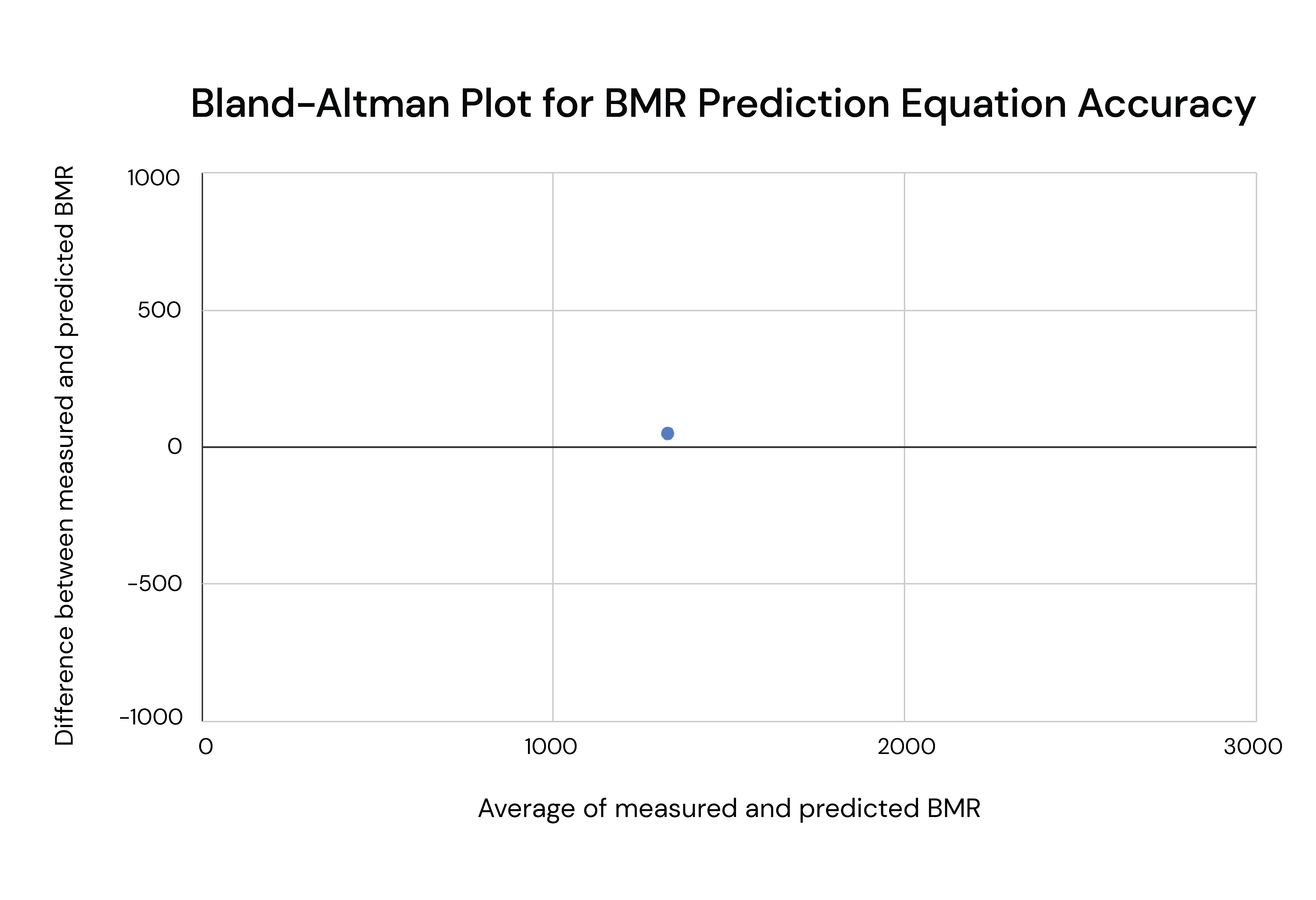
So, if your first subject had a measured BMR of 1300 calories, and a predicted BMR of 1350 calories, the average of their measured and predicted BMRs would be 1325 calories (x-coordinate), and the difference between their predicted and measured BMRs would be 50 calories (y-coordinate). So, you’d plot the point (1325,50) on your graph:

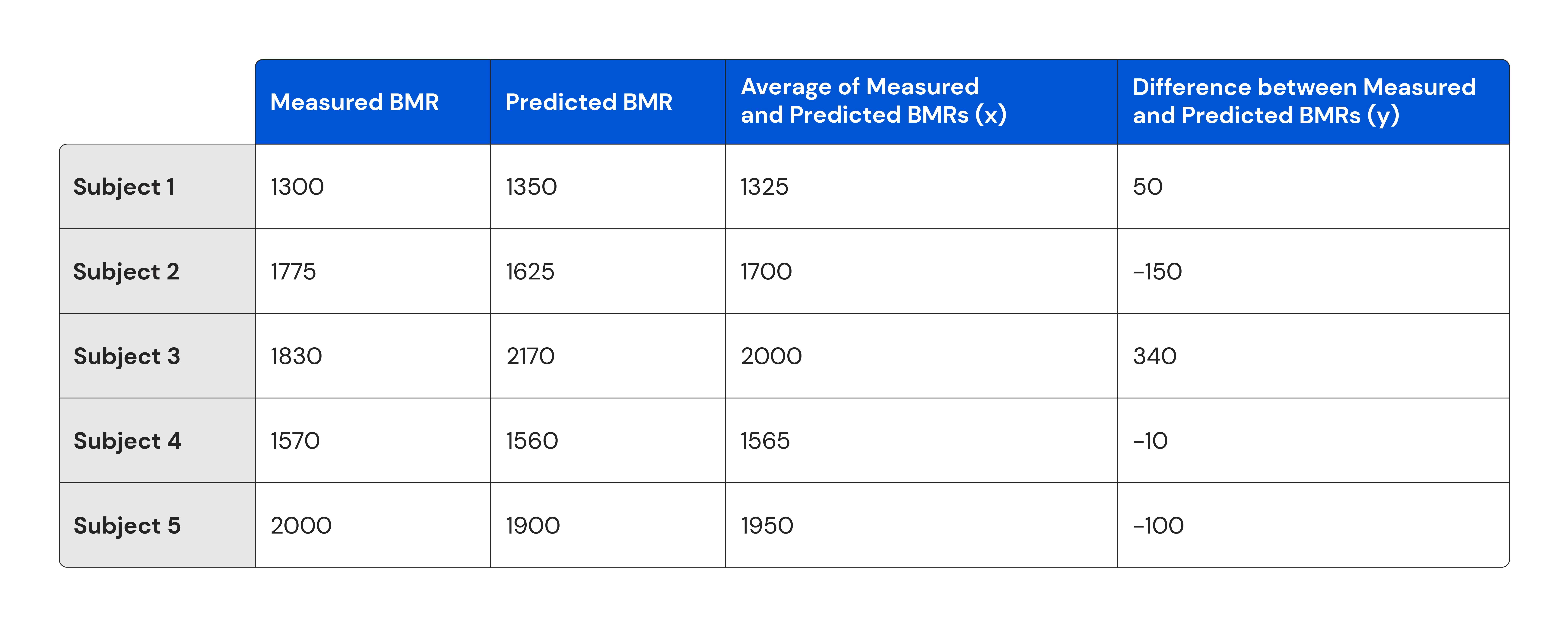
You then collect data on four more subjects, and these are the results:

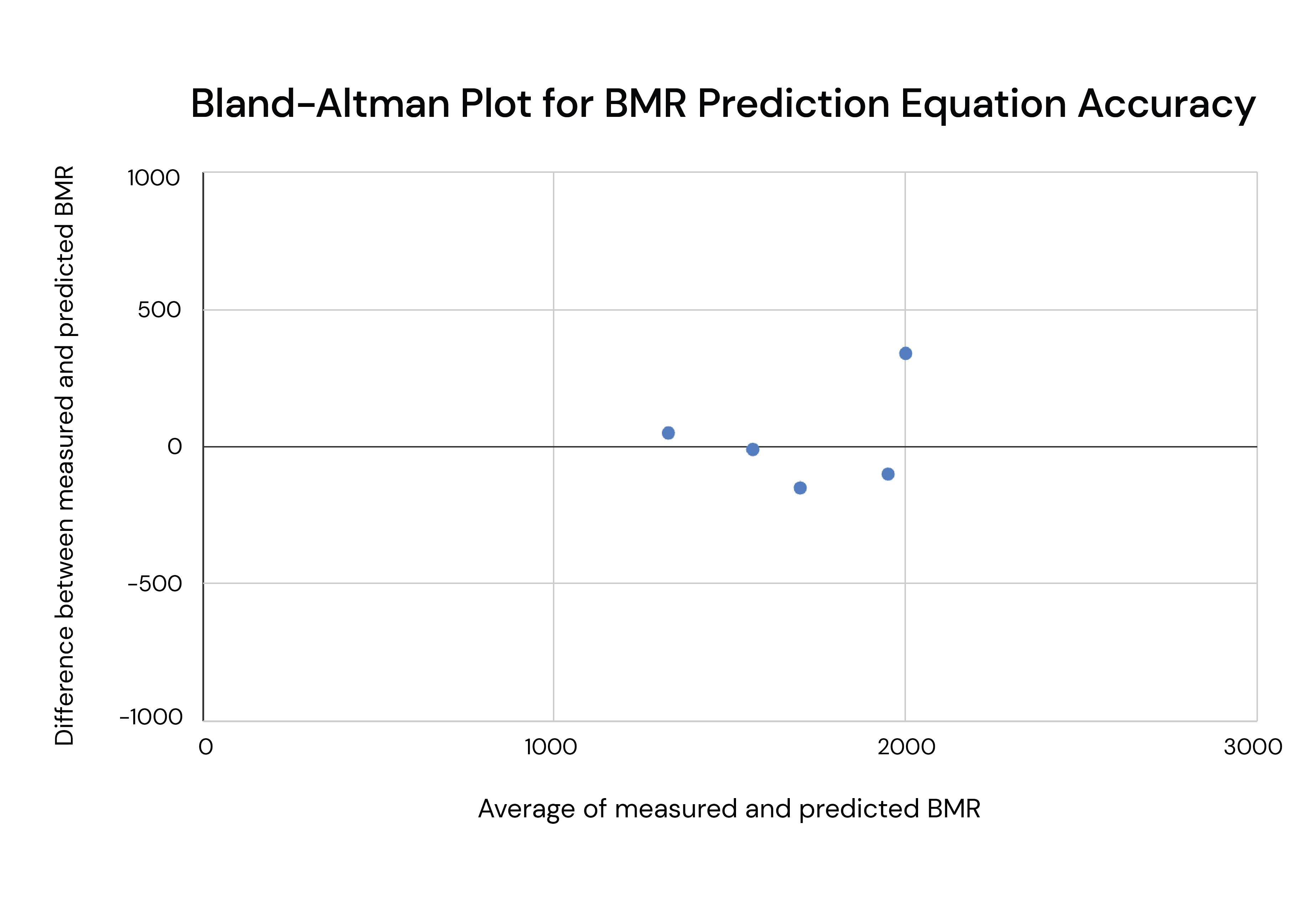
Here’s how your Bland-Altman plot would look after graphing those new points:

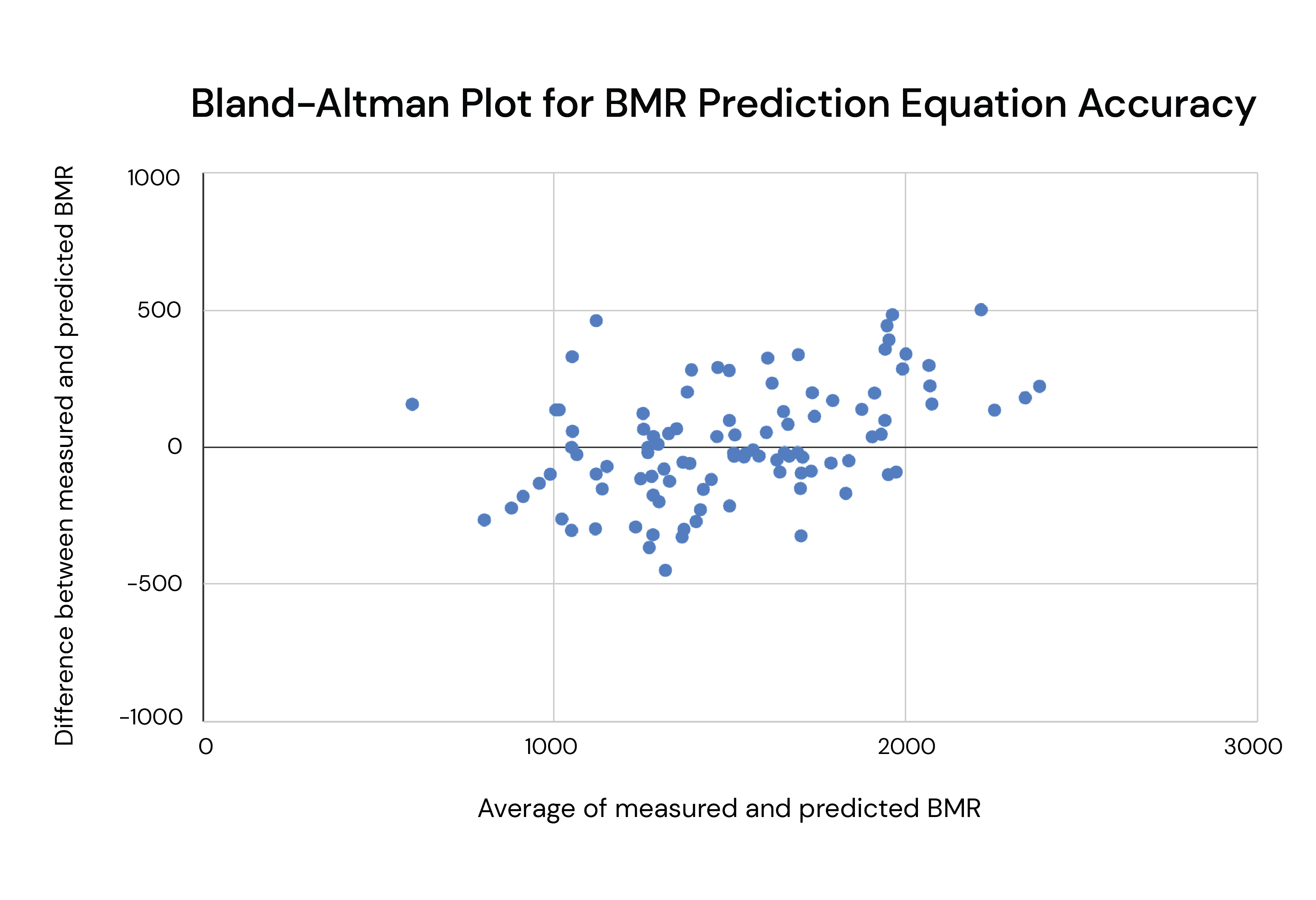
From there, you just repeat the process until you’ve collected and graphed all of your data. Here’s how it might look after you collect and plot the data for 100 subjects:

We’re almost there! There are just two more things to add to our Bland-Altman plot. First, we need to calculate the average prediction error. To do this, we just average all of the y-coordinate values (differences between measured and predicted BMRs). For this dataset, the average error is about 15 calories. In other words, the theoretical BMR prediction equation we’re evaluating in this example overestimates peoples’ BMRs by about 15 calories, on average. After calculating the average prediction error, we graph it as a horizontal line on our Bland-Altman plot:

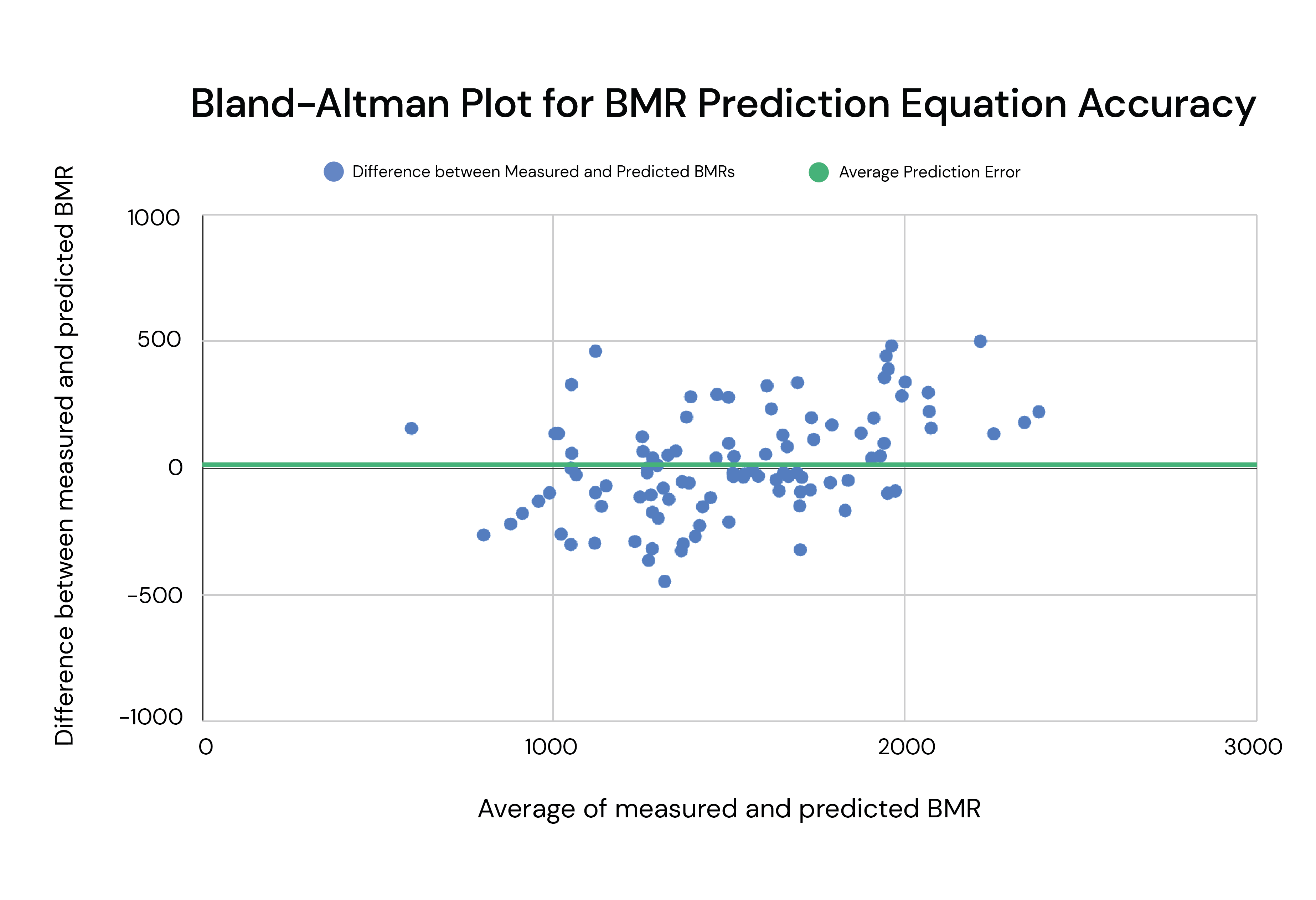
Finally, we calculate the limits of agreement. Limits of agreement tell you the range in which 95% of your data points should fall. So, to find your limits of agreement, you first calculate the standard deviation of your prediction errors. In this case, the standard deviation is about 207 calories. 95% of your data should fall within ±1.96 standard deviations from the mean, so you just multiply the standard deviation by 1.96 (207 x 1.96 = 406 calories, in this case), and then add and subtract the resulting value from your average prediction error to find the top and bottom of your limits of agreement. So the top end of the limits of agreement would be 15 + 406 = 421 calories, and the bottom end of the limits of agreement would be 15 – 406 = -391 calories.

After calculating the limits of agreement, we graph them as horizontal lines as well:

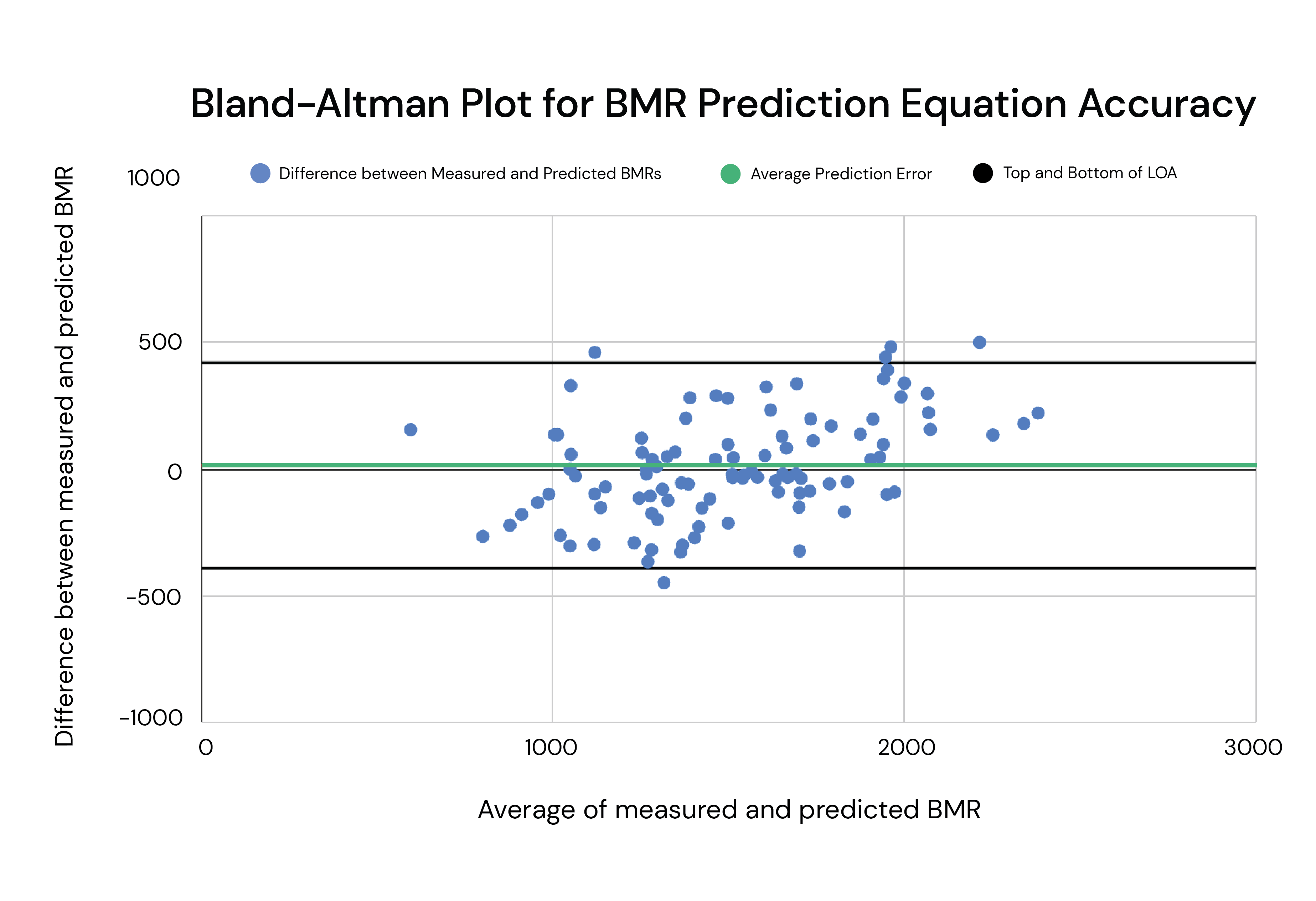
And…that’s about it! You could also plot a trendline to assess if a particular equation systematically over- or under-estimates BMRs for people with higher or lower BMRs, but that’s not necessary for our purposes here. For this article, you just need to understand how limits of agreement are calculated, and what they represent. In this case, the limits of agreement tell you the range of the normal, run-of-the-mill differences between measured and predicted BMRs.

In this example, the limits of agreement span from -391 calories to 406 calories, which would mean that this theoretical BMR equation could underestimate BMR by up to 391 calories, or overestimate BMR by up to 406 calories. So, if your BMR was predicted to be 1500 calories after accounting for things like age, weight, sex, and body composition, that would mean there was a 95% chance your actual BMR was somewhere between 1109 and 1921 calories: an 812 calorie range ³ You can also interpret it the other way as well. If your actual BMR is 1500 calories, the prediction equation has a 95% chance of estimating your BMR to be somewhere between 1109 and 1921 calories. That’s technically the more correct way to interpret it, but I just find that people almost always find that interpretation to be more confusing, and the functional takeaway is similar either way unless there’s a large mean prediction error.

Stated another way, if two people with similar characteristics (age, weight, sex, body composition, etc.) were both predicted to have a BMR of 1500 calories in this theoretical example, it would be entirely possible for one to have a “fast metabolism,” and actually have a BMR of 1900 calories, and the other to have a “slow metabolism,” and actually have a BMR of 1150 calories.

Just to reiterate, the limits of agreement circumscribe 95% of outcomes, all of which are within 2 standard deviations of the mean. In other words, in a room with 14 people, there’s a ~50/50 chance that one of them would have a fast or slow enough metabolism to fall outside of the limits of agreement. The limits of agreement tell you about the totally normal amount of variability observed within a population. You don’t need to be a 1-in-10,000 outlier to bump up against the limits of agreement.

So, that’s how I’ll be evaluating the inter-individual variability of BMRs, when controlling for the relevant covariates: I’ll just be noting the range of the limits of agreement in studies that assess the accuracy of BMR prediction equations. 

Digging into the research: How much do BMRs vary between individuals?

There’s an absolute mountain of research on this topic, but I’ll just focus on three studies that should illustrate the point. All three evaluate several different BMR prediction equations, so no one can accuse me of cherry-picking to make my point. In fact, I selected three of the strongest studies to refute my point: All three demonstrate particularly optimistic scenarios for BMR equations. One evaluates the performance of 26 different equations to figure out which one performs best in various populations, and two develop their own equations that are designed to perform optimally in a single population of subjects (which is the best-case scenario for making a particular equation look particularly accurate).

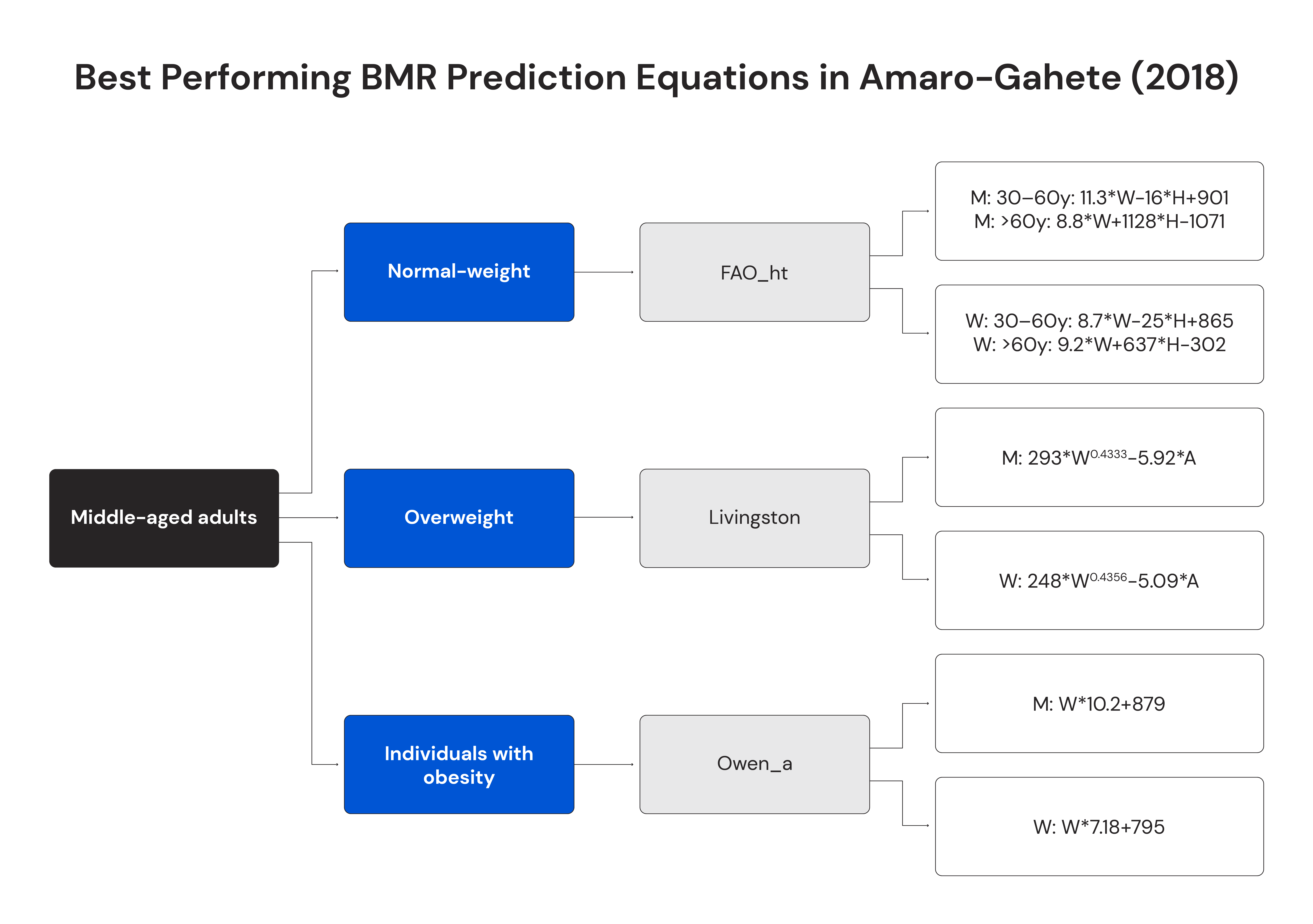
We’ll start with a 2018 study by Amaro-Gahete and colleagues. The researchers recruited a total sample of 73 middle-aged subjects, split them out by BMI status (normal weight, overweight, and obese), and tested 26 different BMR prediction equations to see which one performed best in each population. So, from the outset, this study was virtually guaranteed to produce some unrealistically optimistic outcomes: The best-performing equations in a particular sample will almost necessarily perform worse in a different or broader sample. So, how do the best-performing equations look for each population?

Well, the best-performing equation in normal-weight individuals was the version of the FAO equation that incorporates height; the best-performing equation in overweight individuals was the Livingston equation; and the best-performing equation in individuals with obesity was one of the versions of the Owen equation:

And, here’s how each of the hand-picked equations performed:

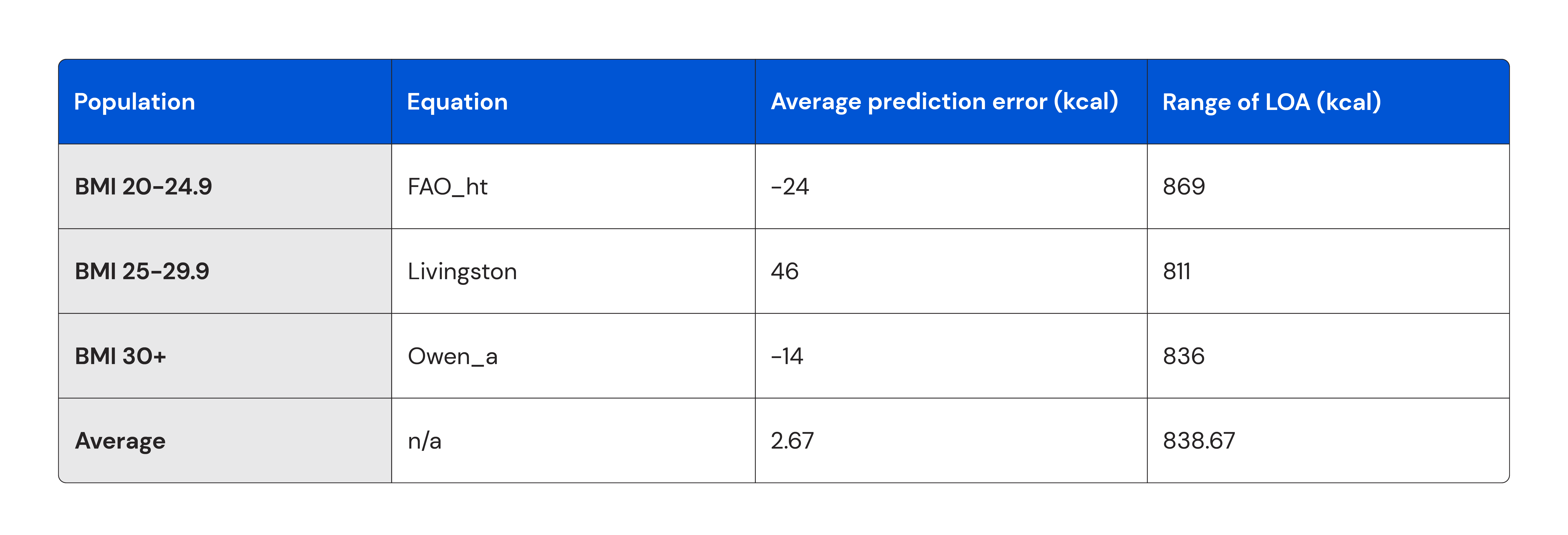
The study didn’t present Bland-Altman plots for each of these equations, but here’s an illustration of how one would look, using synthetic data with the same characteristics as the “Average” row above:

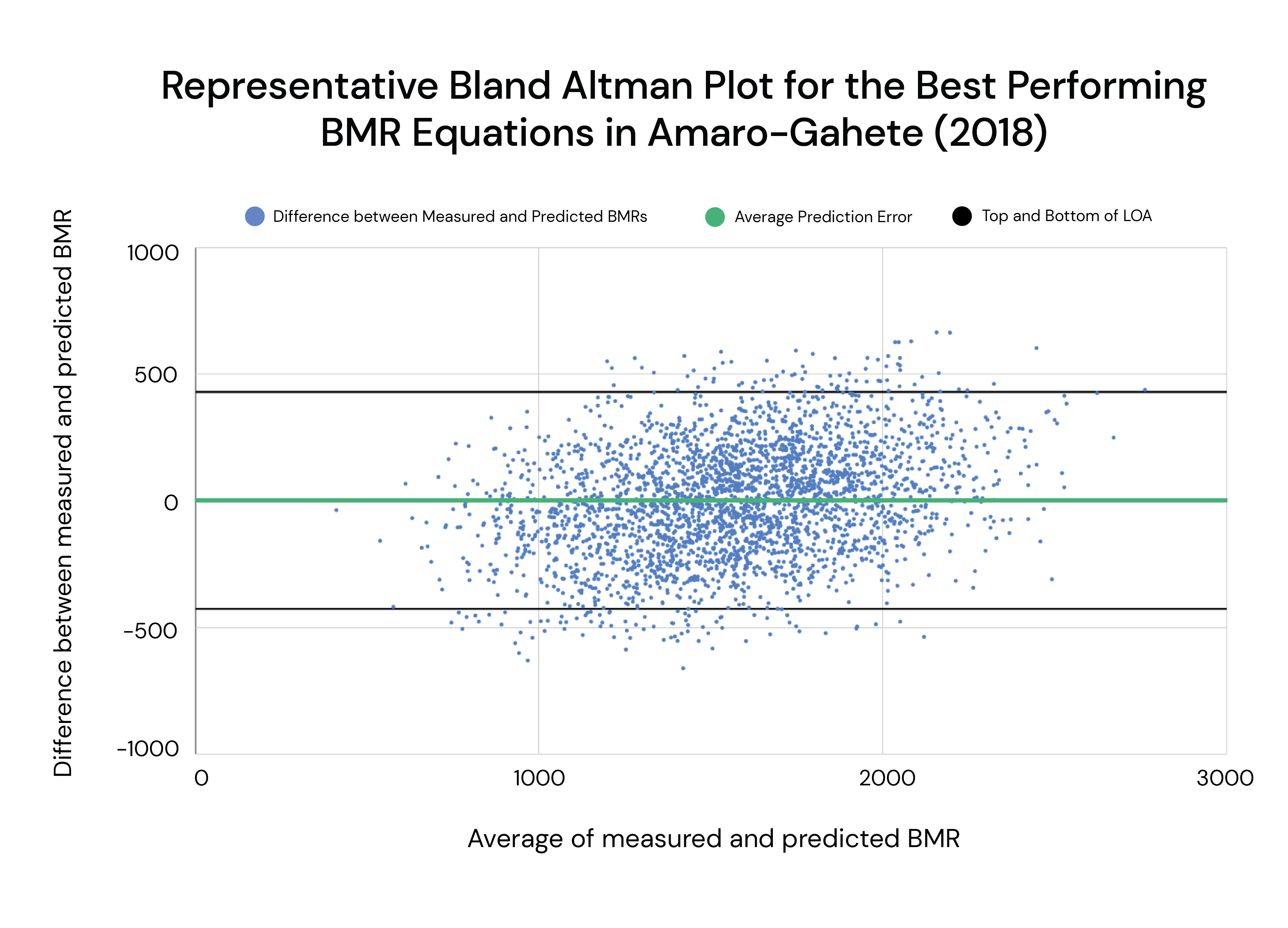
Of note, the tightest limits of agreement for any equation and any population was 666 calories (the Owen_b equation in overweight individuals), but the average prediction error for that equation was pretty bad: it underestimated BMR by an average of 251 calories. Conversely, the widest limits of agreement spanned 1354 calories (the De la Cruz equation, also in overweight individuals). On average, across all equations and all populations, the limits of agreement covered a range of 843 calories.

Moving on, we have a 2019 study by Tinsley and colleagues. In this study, the researchers compared the performance of 11 BMR equations in a pretty homogeneous sample of lean, muscular physique athletes (17 males and 10 females). In general, BMRs should have less inter-individual variability in more homogeneous populations. Furthermore, the researchers developed a new equation that was generated for the specific population included in the study. So, the deck was stacked in favor of generating a best-case scenario for the accuracy of BMR prediction equations.

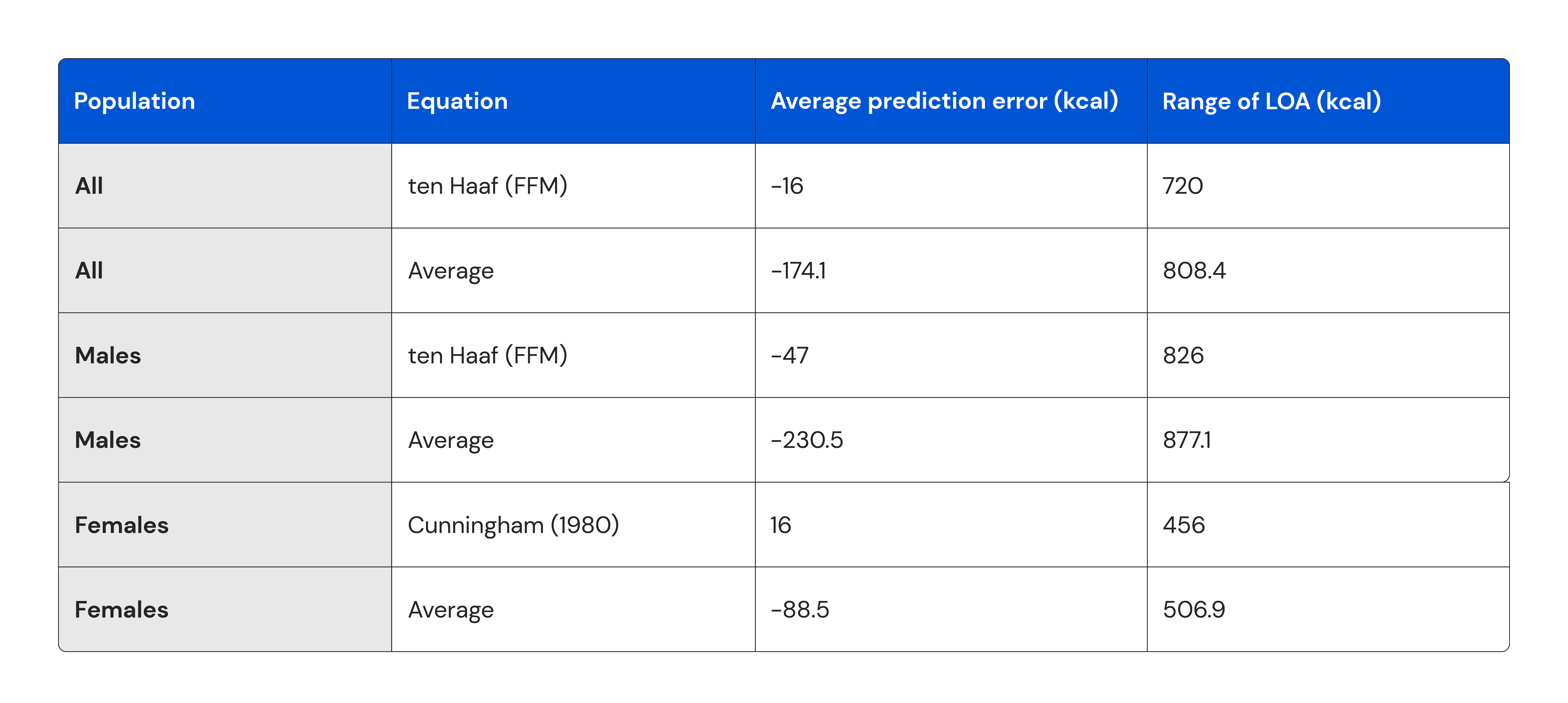
In the full sample, the best-performing equation (the ten Haaf equation) underestimated BMRs by 16 calories, on average, with limits of agreement spanning a total range of 720 calories.

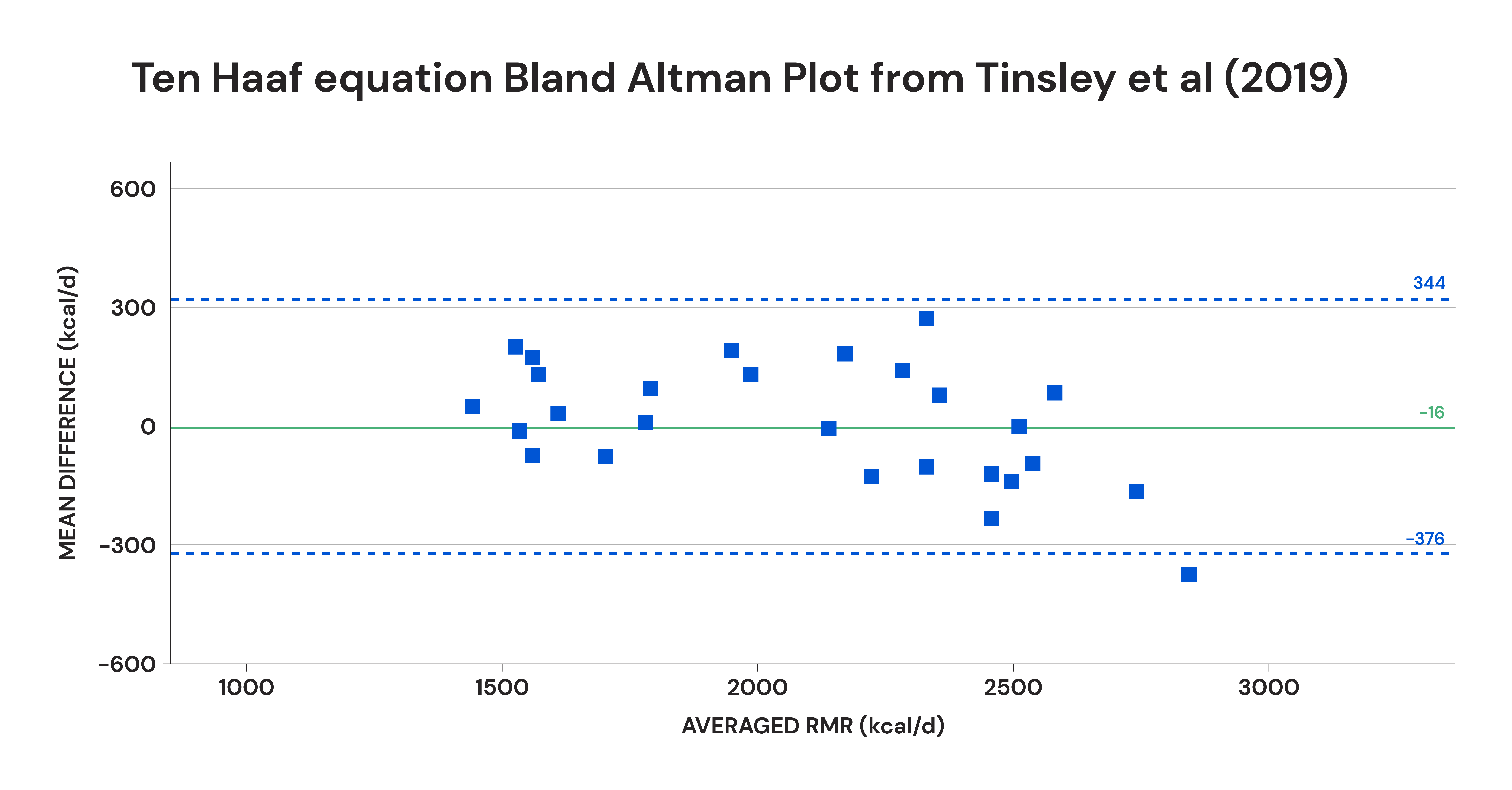
The ten Haaf equation also performed best for the subsample of male subjects, underestimating BMR by an average of 47 calories, with limits of agreement spanning an 826 calorie range. Finally, the subsample of 10 female subjects had literally the most predictable BMRs I’ve ever seen reported in the literature, with the tightest limits of agreement I’m aware of. The best-performing equation (the 1980 version of the Cunningham equation) overestimated their BMRs by an average of 16 calories, with limits of agreement spanning a range of just 456 calories.

The table below shows the best-performing equation in each population, and the average performance of all 11 equations that were evaluated:

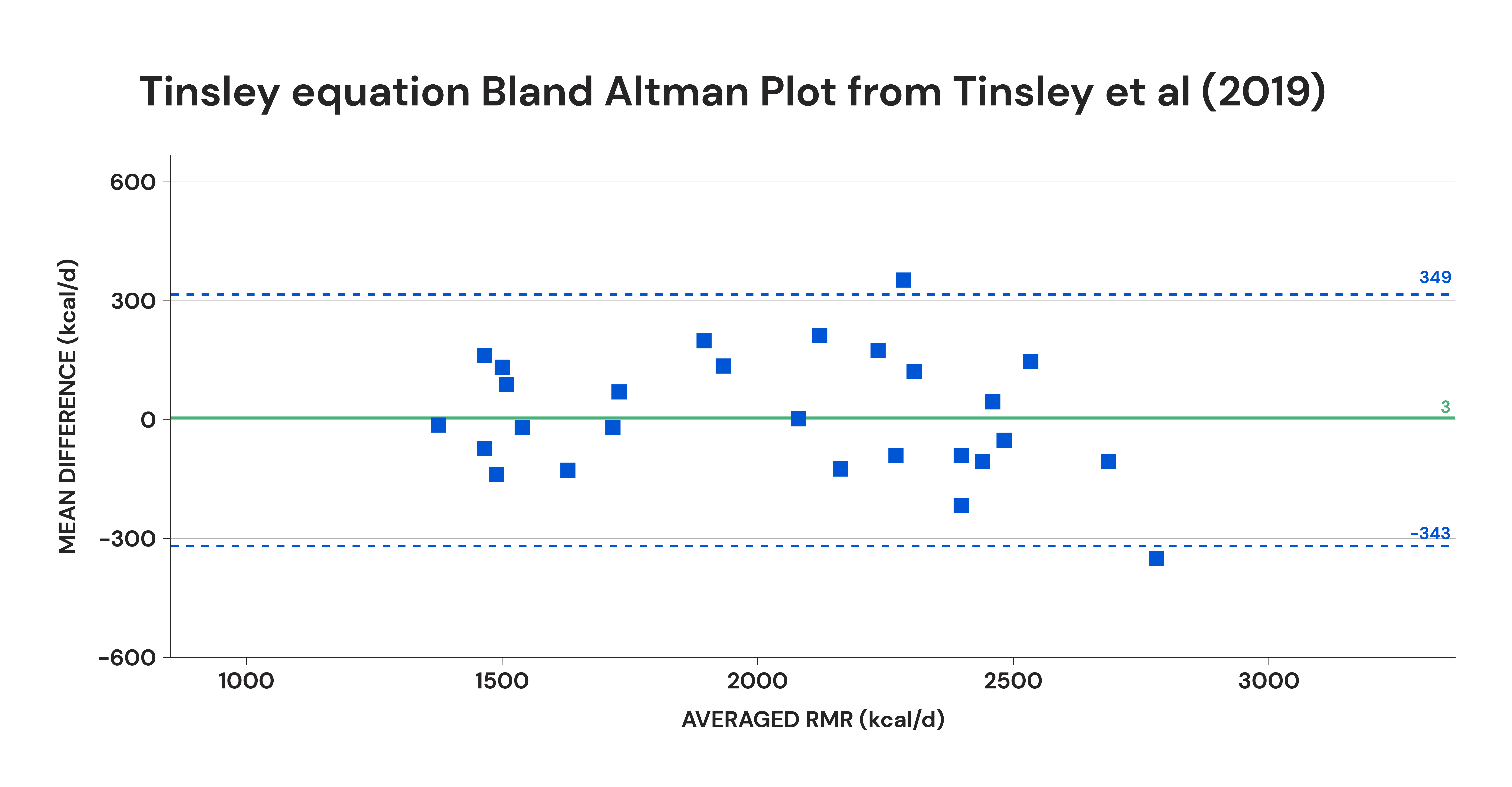
Finally, as mentioned previously, the researchers created a brand new BMR prediction equation based on the specific sample of physique athletes included in the study. As expected, it performed better than any of the other equations in the full sample, underestimating BMR by just 3 calories, on average, with limits of agreement spanning a range of just 692 calories.

Let’s round things out by looking at a study by Pavlidou and colleagues that’s hot off the presses.

The researchers recruited a sample of 722 subjects (173 males and 549 females), ranging from 18 to 78 years old. In this study, they created and validated a new BMR prediction equation, and compared their new equation to four of the most popular equations (Harris-Benedict, Mifflin-St Jeor, FAO, and Owen).

Validating a new equation is a two-step process. First, you create a new equation based on the data from one sample of subjects. Then, you test how well the equation performs in another sample of subjects. This makes sure that your equation generalizes, instead of simply being over-fit and only performing well in the population it was developed from. In other words, the validation step provides a more accurate assessment of how the equation performs. If you only evaluate an equation in the population it was developed from, you’ll generally wind up with an overly optimistic view of its performance. ⁴Just so it doesn’t sound like I’m ragging on Tinsley and colleagues, they did also validate their new equation, using leave-one-out cross-validation. It’s not worth going into the details here, but the validation method used in the study by Pavlidou is generally considered to be a superior method. Though, given the small sample size they were working with, the validation method used by Tinsley and colleagues was probably the best option available to them. So about three-fourths of the subjects were used to develop the equation, and the remaining one-fourth were used as the validation groups.

Unsurprisingly, the new equation developed by Pavlidou was the best of the bunch, performing better than the other four equations. It overestimated BMR by just 5 calories, on average, with limits of agreement spanning a range of 719 calories.

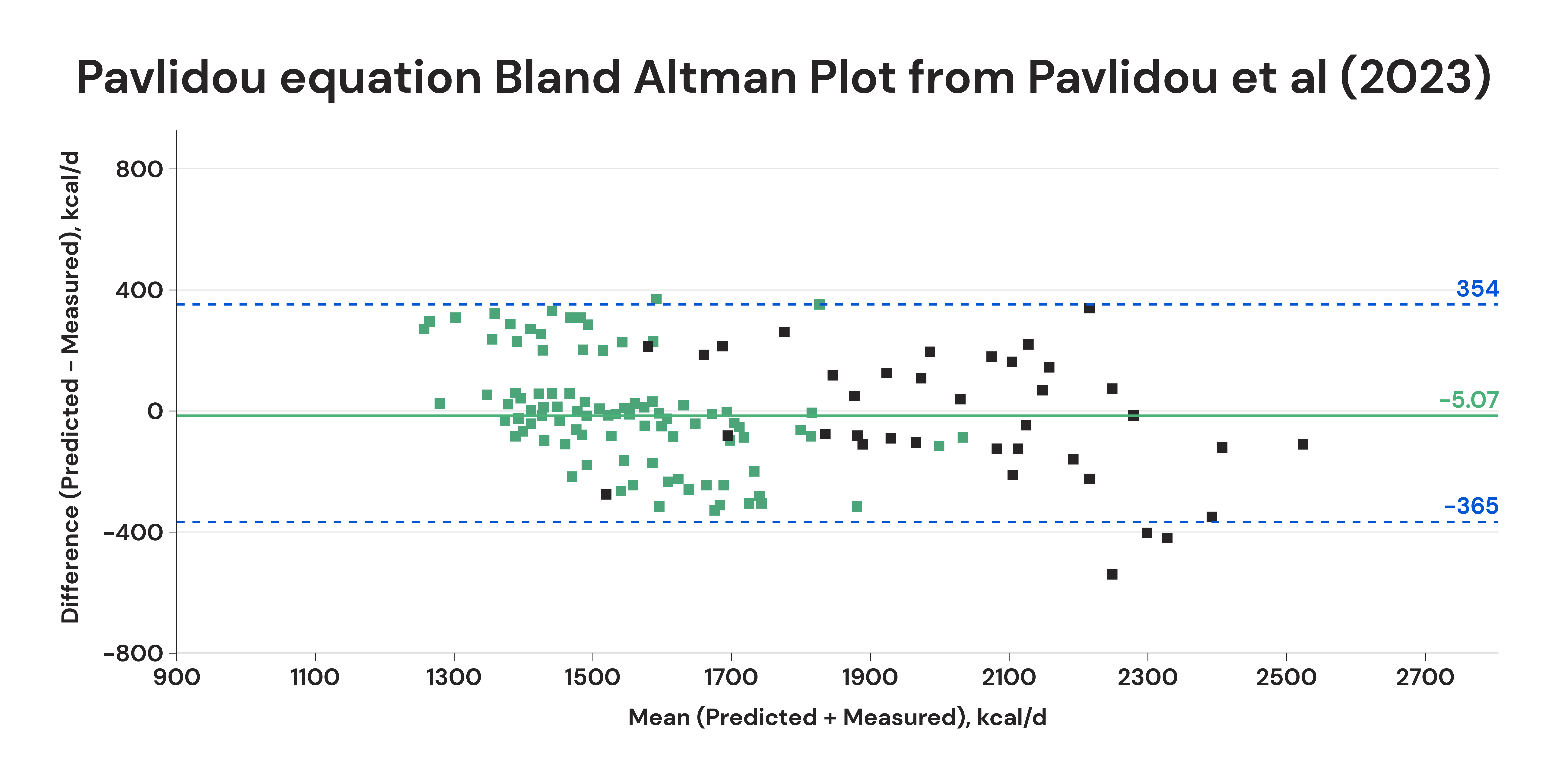
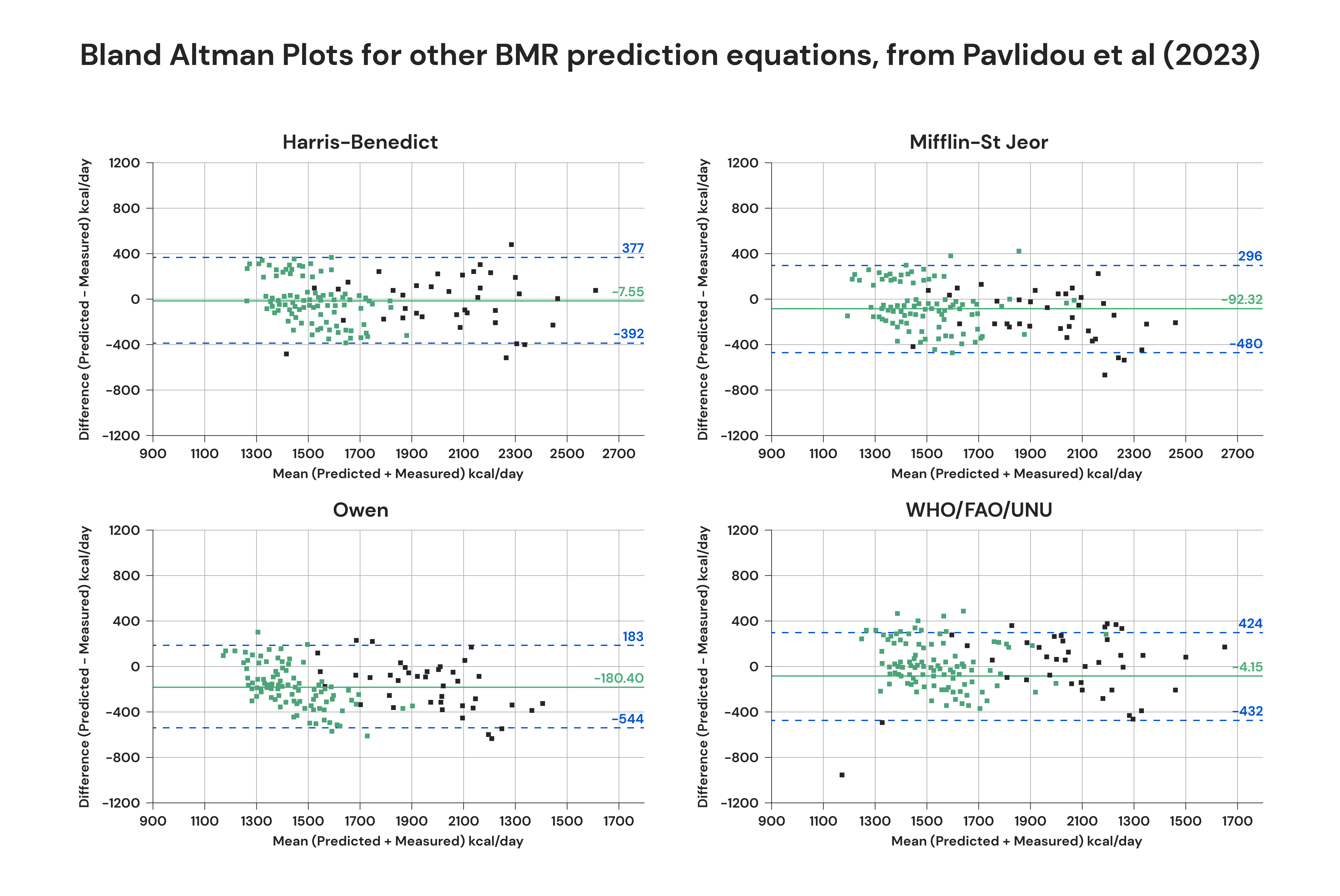
Limits of agreement for the other four equations spanned ranges of 769 (Harris-Benedict), 776 (Mifflin-St Jeor), 727 (Owen), and 865 calories (FAO). However, the average prediction errors for the Mifflin-St Jeor and Owen equations were both pretty large.

I realize that was a lot – a lot of numbers, a lot of graphs, etc. – so let’s briefly summarize the takeaways.

I selected a sample of studies that let us see the upper limits of how well BMR equations can perform, while also showing how well they typically perform.

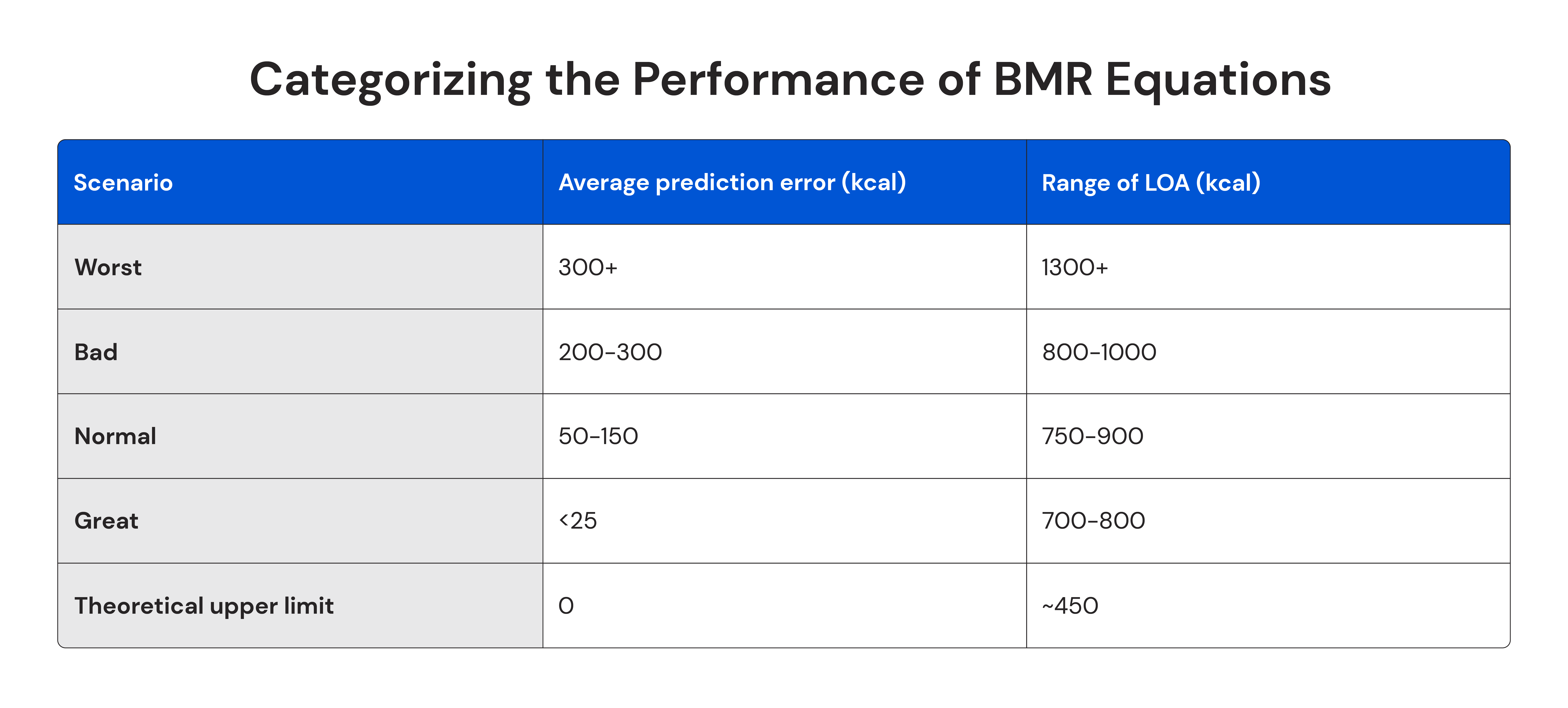
The best-performing equations in each study were equations that were either shown to perform particularly well in a specific sample of subjects, or equations that were specifically created to perform well in the sample of subjects recruited for each study. Those high-performing equations had very low average prediction errors, but still had limits of agreement that covered a ~700-800 calorie range.

The “average” equations in most of these studies mostly had limits of agreement spanning a range of ~750-900 calories, while having average prediction errors of about 50-150 calories.

The absolute worst equations had average prediction errors exceeding 300 calories, and limits of agreement exceeding 1300 calories.

Finally, I think the female subsample in the Tinsley study presents us with a truly pie-in-the-sky scenario, showing how well BMR prediction equations theoretically could perform if you happened to have a sufficiently homogenous population, and happened to pick (or create) the perfect equation for that specific population. However, even in that scenario, the limits of agreement still spanned a range of about 450 calories. In other words, someone with a “fast metabolism” and someone with a “slow metabolism” could still have BMRs that differed by 450 calories per day, even if they were the same age, height, weight, body composition, etc.

Further considerations

If you don’t care much about digging into the minutiae, feel free to skip this section, and scroll down until you see the heading, “What can we do about it?” I want this to be a pretty comprehensive resource, so I’m going to use this section to go down a couple small rabbit holes and respond to a few technical questions I anticipate some readers will have. However, if you don’t feel like getting into the weeds, this section is definitely skippable. There will be several fun nuggets in this section, though.

Why is it so challenging to precisely estimate BMRs?

At first, it may seem a bit surprising that BMRs are difficult to precisely estimate. However, when we go a step deeper, the primary reason is surprisingly simple.

Remember, your BMR is the amount of energy your body burns at rest. So, we can decompose BMR into the amount of energy each organ burns at rest. When you do that, it becomes apparent that your BMR is primarily determined by the BMRs of your internal organs.

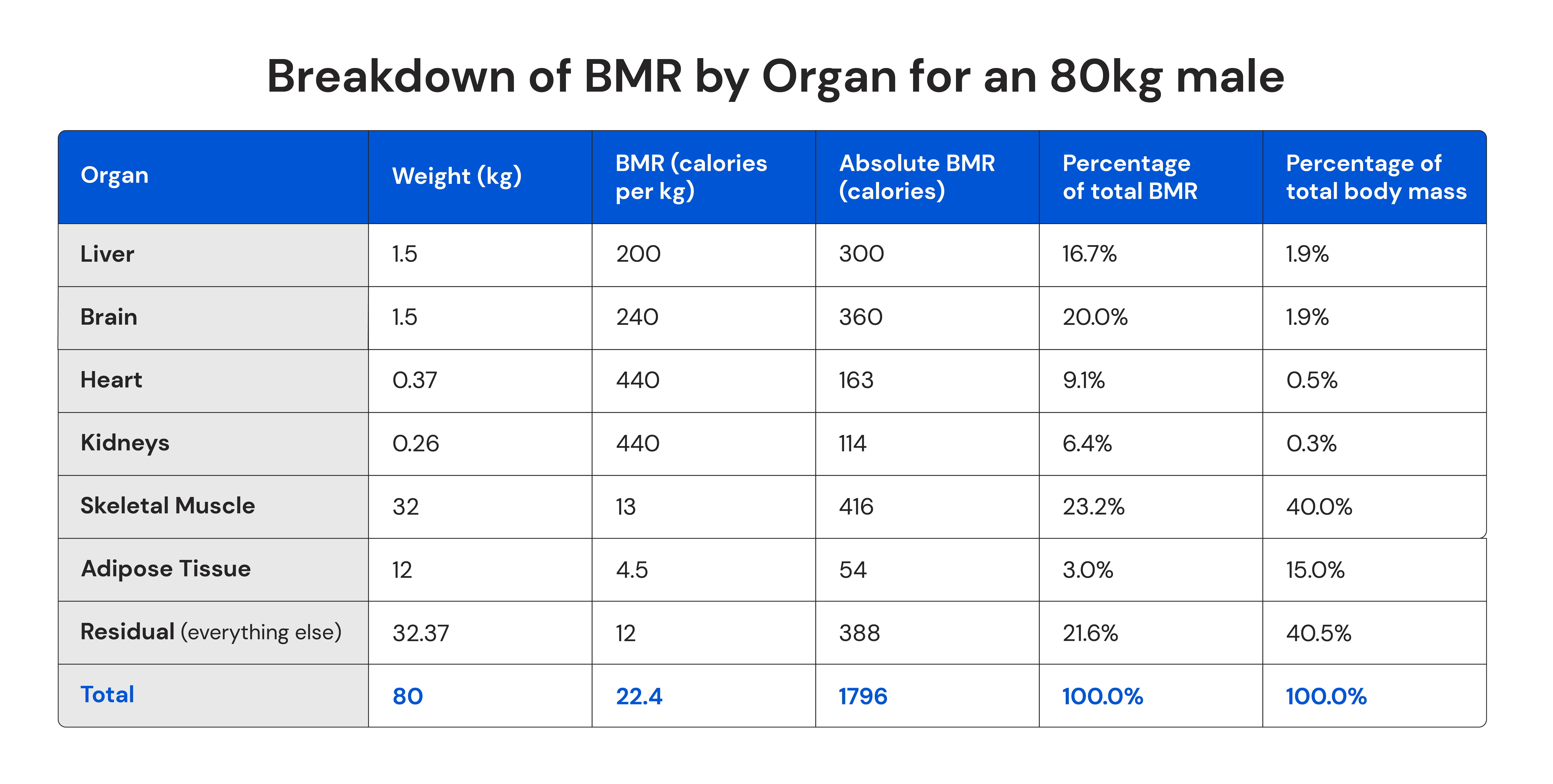
The BMR of skeletal muscle is approximately 13 calories per kilogram, and the BMR of your adipose tissue is approximately 4.5 calories per kilogram. So, let’s assume that we’re estimating the BMR of a young male with pretty normal body composition. We’ll assume that he weighs 80kg, that he has a body fat percentage of 15%, and that 40% of his body mass is comprised of skeletal muscle (which is pretty typical for a male in the general population).

On average, you’d expect him to have a BMR of about 1800 calories. He has 32kg of skeletal muscle burning 13 calories per kilogram at rest, and 12kg of adipose tissue burning 4.5 calories per kilogram at rest. So, his skeletal muscle and fat tissue account for about 470 calories – about a quarter of his total BMR. The other three quarters is accounted for by his other organs – his brain, heart, liver, kidneys, etc. Those organs each account for a small percentage of his total body mass, but they’re also way more metabolically active per unit of mass.

For instance, each kidney weighs about 130g, on average, but kidneys have a BMR of about 440 calories per kilogram. So, his kidneys, which only account for 0.325% of his total body mass, burn about 114.4 calories per day at rest – more than 6% of his total BMR. Similarly, the brain and liver (about 1.5kg apiece) have basal metabolic rates of about 240 and 200 calories per kilogram, respectively. So, they only account for about 3.75% of his total body mass, but they burn about 660 calories per day at rest, accounting for more than a third of his BMR, and more total calories than his adipose tissue and skeletal muscle mass combined, despite the fact that adipose tissue and skeletal muscle account for 55% of his total body mass.

Because of how metabolically active your organs are, two things could dramatically increase the unpredictability of BMRs: variability in organ mass, and variability in organ-specific BMRs.

I’m sure you can see where this is going:

Organ mass and organ-specific BMRs vary considerably between individuals.

Variability in Organ Mass

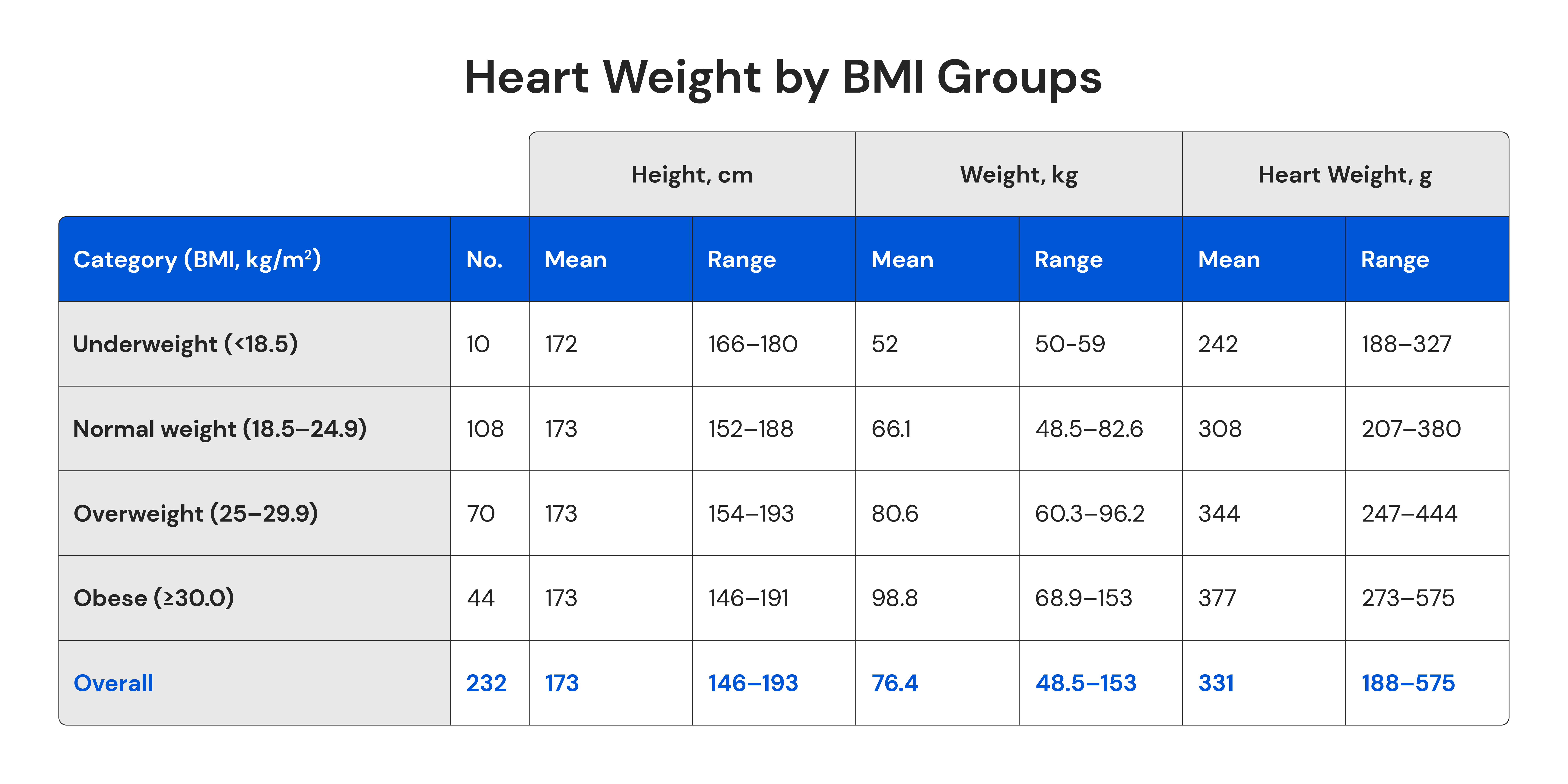
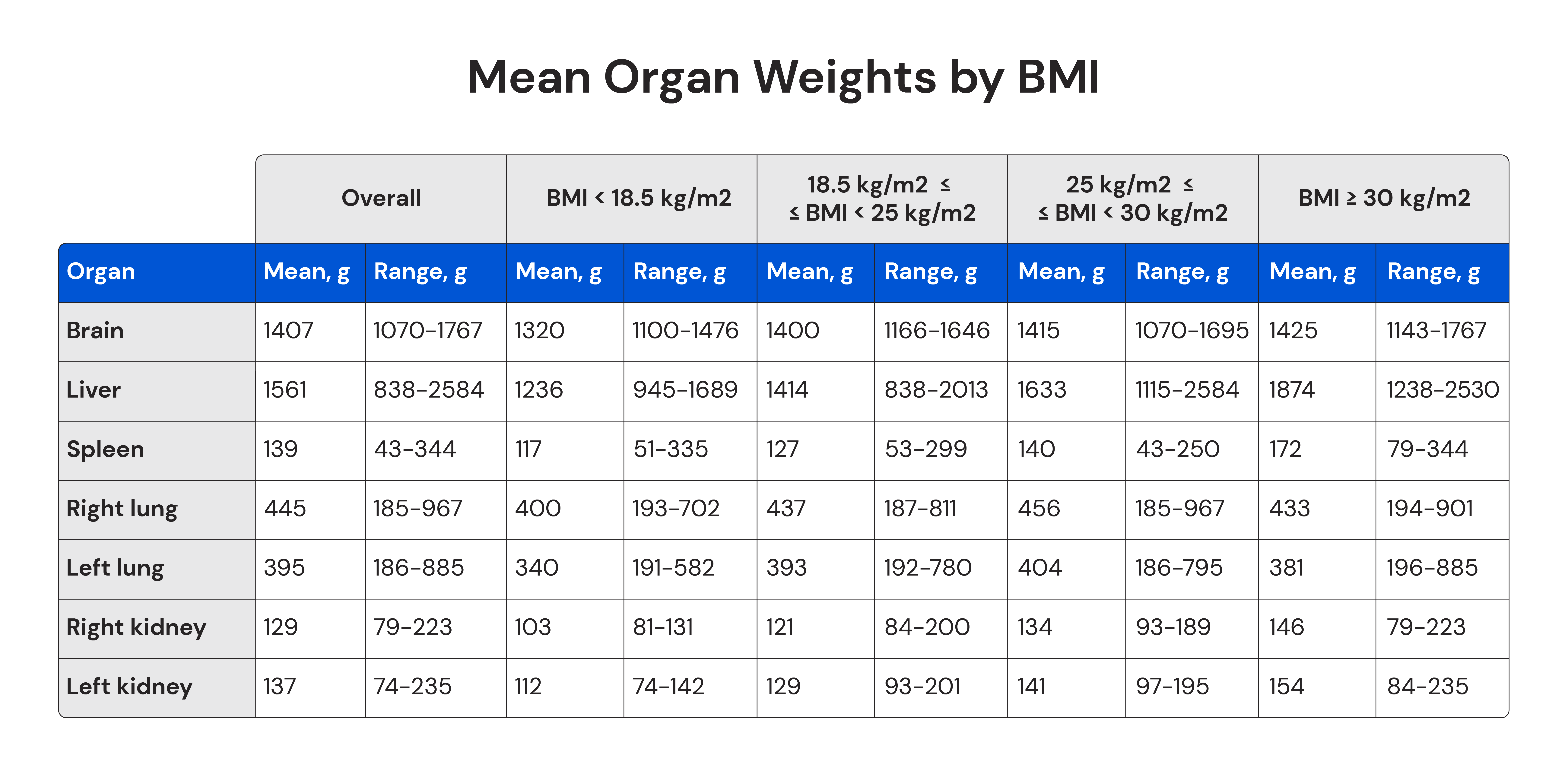
Starting with organ mass, researchers Molina and DiMaio published autopsy studies detailing the normative ranges for organ masses in men (one, two) and women (one, two) in 2012 and 2015, respectively. They specifically assessed people with no known diseases and no visual indications of organ abnormalities, in order to assess the normal range of organ sizes, barring pathologies that make specific organs grow or shrink.

Here were the results for men:

And here were the results for women:

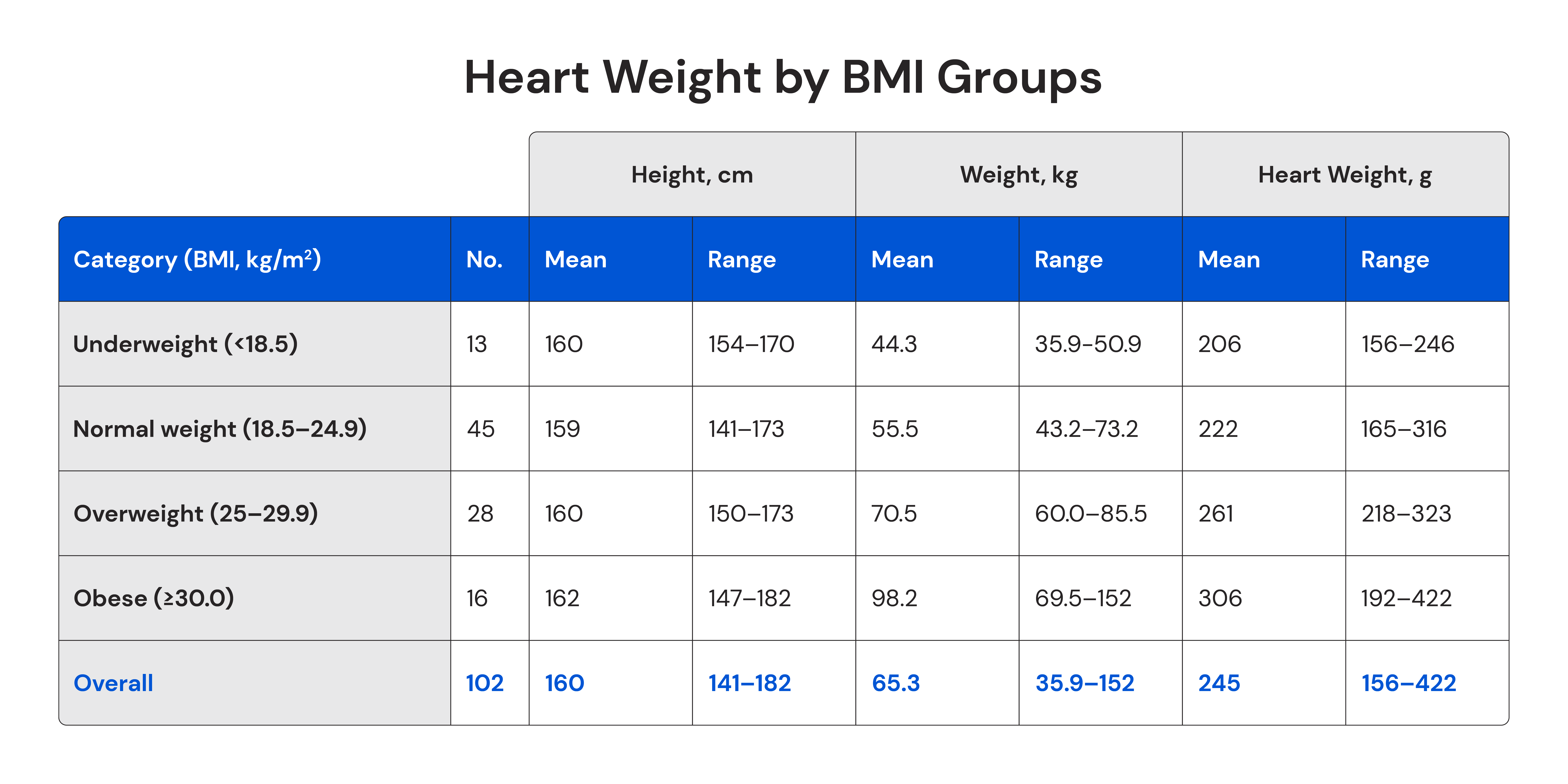
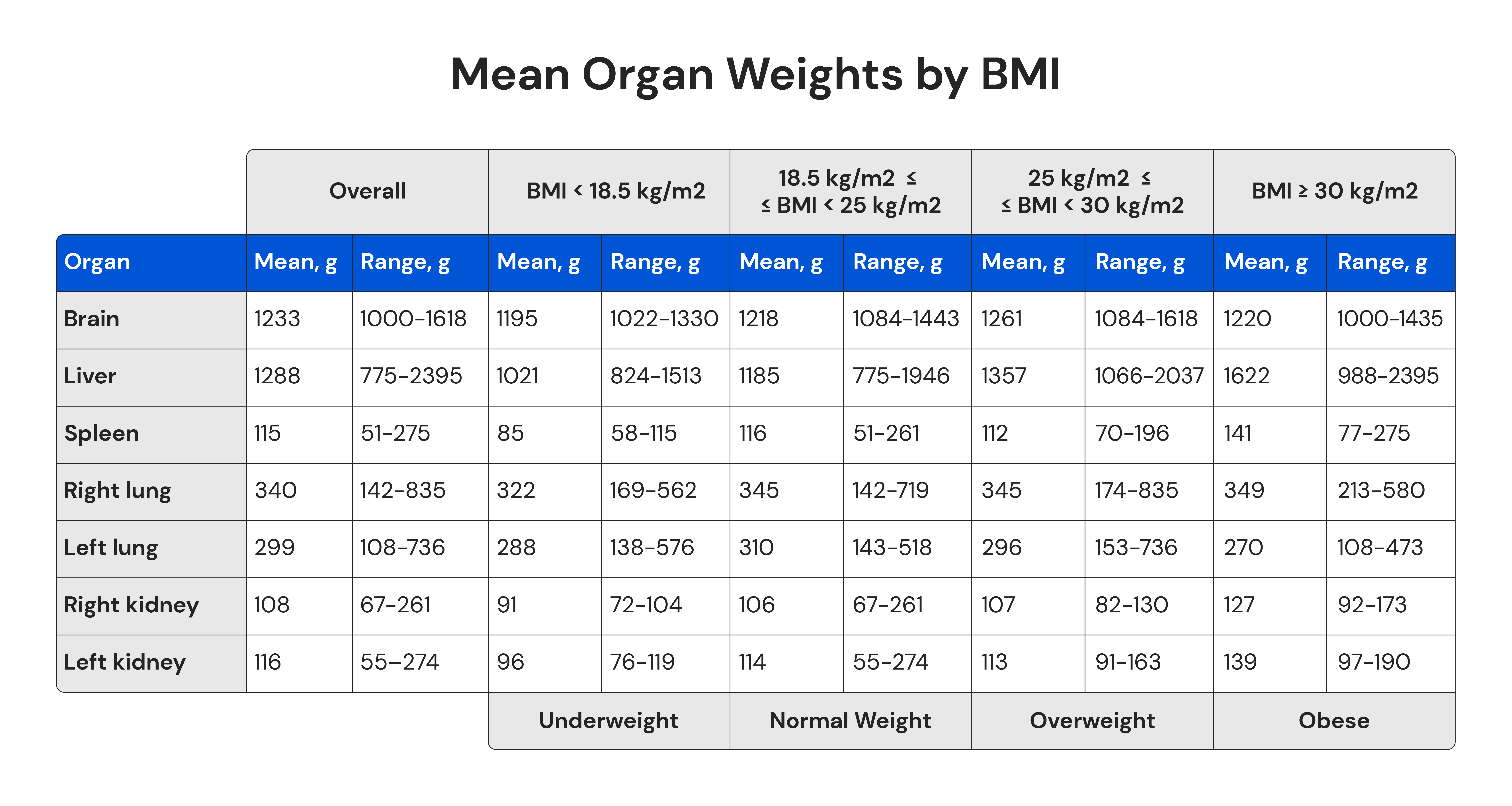
As you can see, organ mass varies considerably between individuals. Heart, liver, and kidney mass all vary within 2-4-fold ranges (i.e. the heaviest organs are 2-4 times heavier than the lightest organs). Brain mass has a bit less variability, but the largest brains are still 60-70% larger than the smallest brains. Conversely, spleen mass varies within an enormous 5-8-fold range.

Furthermore, organ masses are inherently difficult to predict without having a way to look inside the body. Just to illustrate, female heart mass is correlated with height, body mass, and BMI, but they’re all fairly rough correlations. The strongest association is between heart mass and body mass, but variation in body mass still only explains about 66% of the variation in heart mass. In more concrete terms, a 70kg woman could have a heart that weighs less than 200g, or nearly 300g.

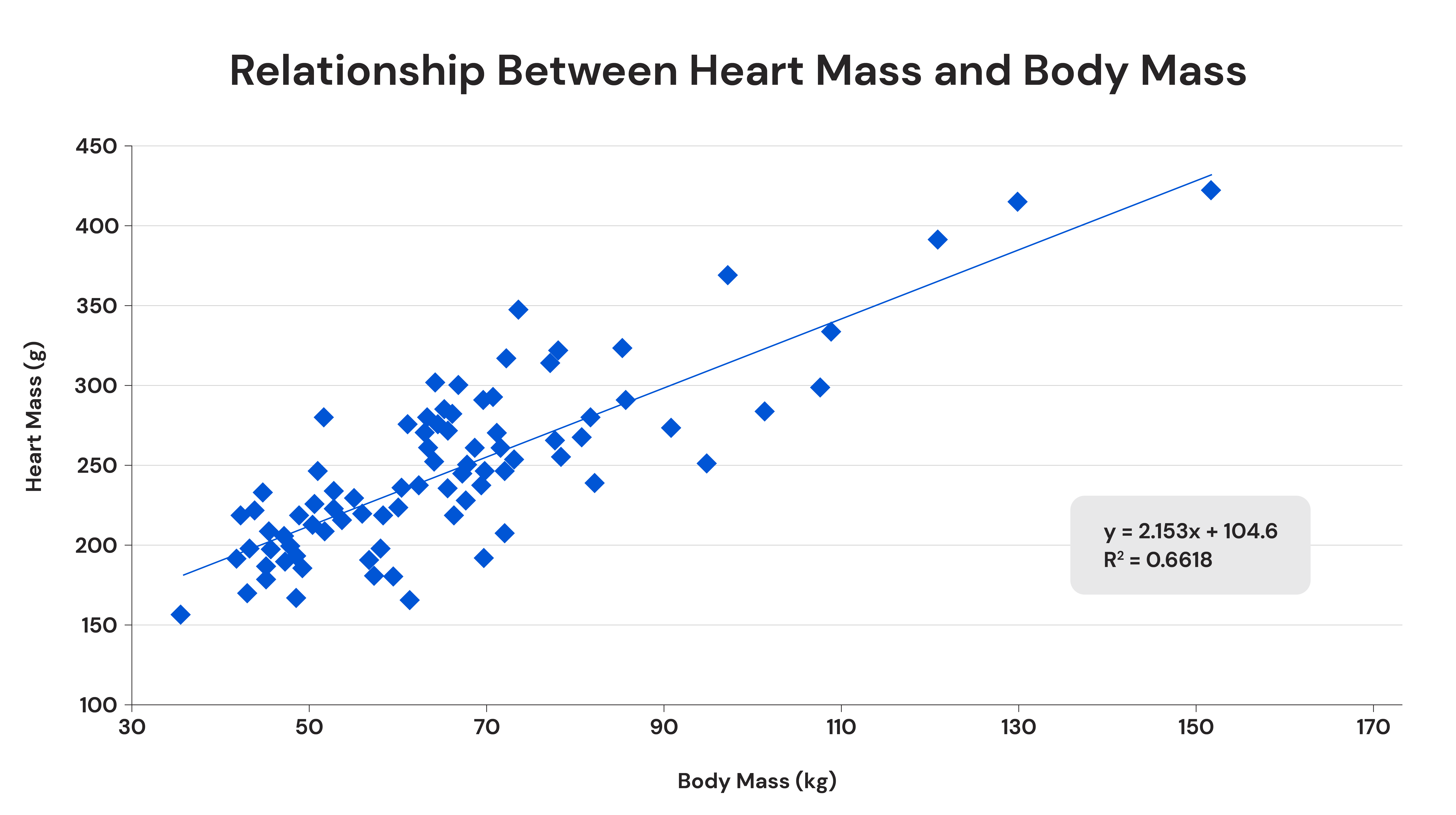
That’s actually the best-case scenario for predicting the mass of an organ based on body size. The masses of other organs are also associated with height, weight, and/or BMI, but all of those associations are even weaker. Body mass explains about 66% of the variance in heart mass, but only 48% of the variance in liver mass, 25-27% of the variance in kidney mass, and even less of the variance of all other organs assessed.

So, here’s the problem:

1. Your organs (outside of skeletal muscles and adipose tissue) are responsible for about three quarters of your BMR.
2. Variation in organ mass can have a very large impact on BMR, because of how metabolically active organs are per unit of mass.
3. We cannot predict organ mass with any reasonable degree of accuracy based on easily observable individual characteristics.

Just to illustrate, if your organs were 50% larger or small than normal for your height, age, weight, sex, etc. (which is comfortably within the realm of normal variability for most major organs, other than the brain), your BMR would likely be about 37.5% higher or lower than would be predicted based on your easily observable demographic and anthropometric characteristics.

However, it gets even worse.

Variability in Organ-Specific BMRs

In the prior section, I discussed the impact of organ size and BMR on total BMR, but I used roughly average values for organ-specific BMRs. However, organ-specific BMRs also have considerable variability. 

It’s very challenging to directly measure the BMR of individual organs, but a 2010 study by Wang and colleagues used an interesting and sophisticated method to estimate the range of organ-specific BMRs.

In short, the researchers:

1. Measured total BMR for each subject.
2. Performed MRI scans to estimate the volume of each organ with a high degree of precision.
3. Estimated the mass of each organ, given the volume estimates and known densities of each organ.
4. Generated BMR estimates for each subject using the typical organ-specific BMRs proposed by Elia and Schimmel (200kcal/kg, 240kcal/kg, 440kcal/kg, 440kcal/kg, 13kcal/kg, 4.5kcal/kg, and 12kcal/kg for the liver, brain, heart, kidneys, skeletal muscles, adipose tissue, and residual component, respectively).
5. Estimated individual organ-specific BMRs via regression, based on the differences between predicted and measured BMRs.

Basically, if you know the mass of each organ, and the specific metabolic rate of each organ, you should be able to perfectly predict BMR (with some allowances for measurement error, of course). Therefore, if you know the mass of each organ, but you only have group-level averages for organ-specific metabolic rates, differences between measured and predicted BMRs should be primarily attributable to variability in organ-specific metabolic rates – this study was designed to estimate that variability.

First of all, this study beautifully illustrates my point from the last section: BMRs are hard to predict accurately due to a) variability in organ mass and b) the inherent unpredictability of organ masses. Since the researchers in this study were able to estimate organ masses very precisely via MRI, they were able to predict BMRs far more accurately than any standard BMR prediction equation, even when initially assuming that there was no variability in organ-specific metabolic rates. The average prediction error was just 13 calories, and the limits of agreement spanned a range of just 318 calories. In other words, the precision of their BMR estimates was 2-4 times higher than the precision of BMR estimates derived from factors like height, weight, age, sex, body composition, etc. This increase in precision should be primarily attributable to the precise estimates of individual organ masses, instead of needing to use a formula that (tacitly) assumes that organ mass basically scales 1:1 with body size.

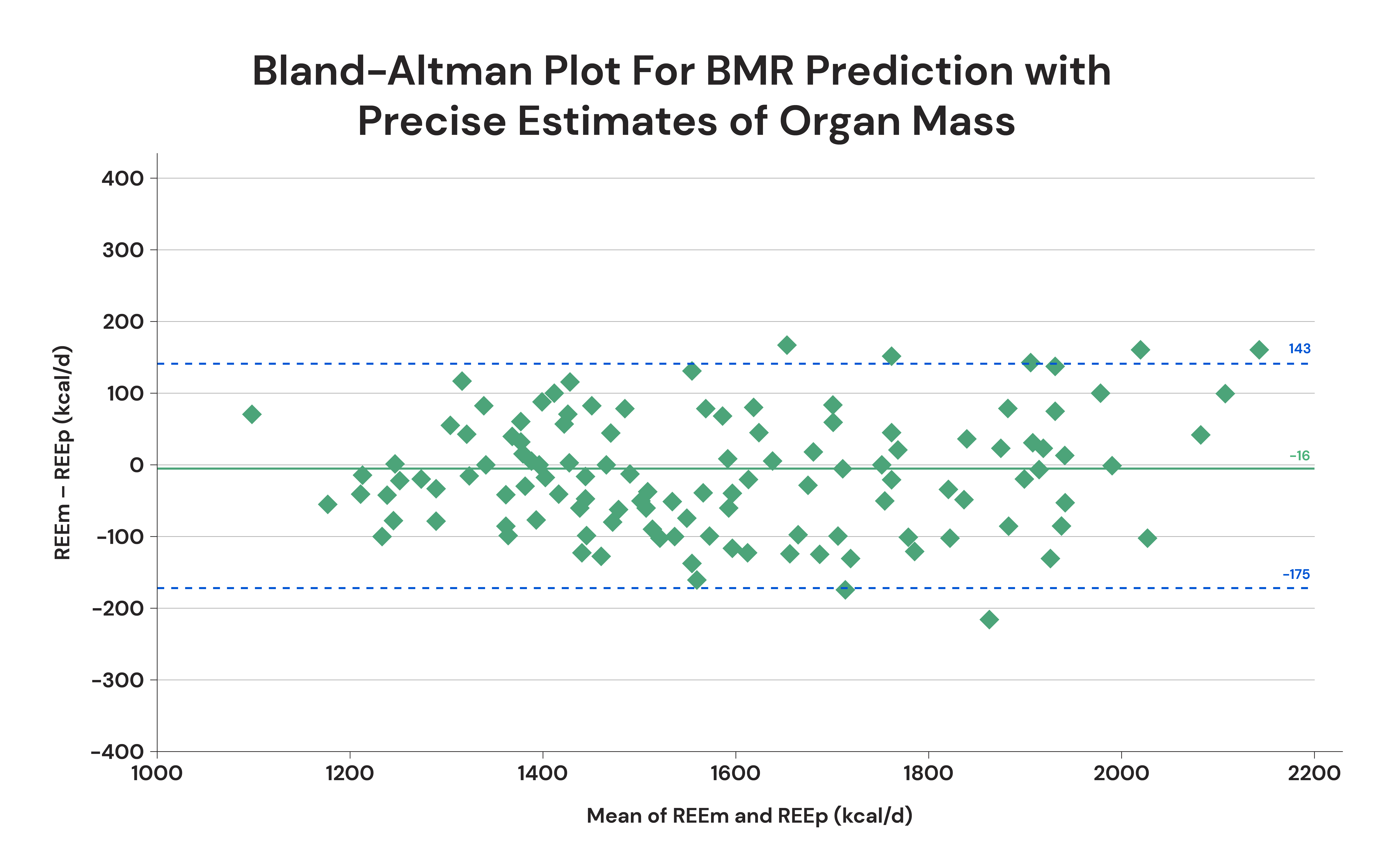
From there, organ-specific BMRs were estimated. In general, the results suggested that organ-specific BMRs span a range of ±10% above or below the average for each age group. In other words, if the average BMR of the liver was 200kcal/kg, 95% of individuals should have liver-specific BMRs ranging from 180-220kcal/kg.

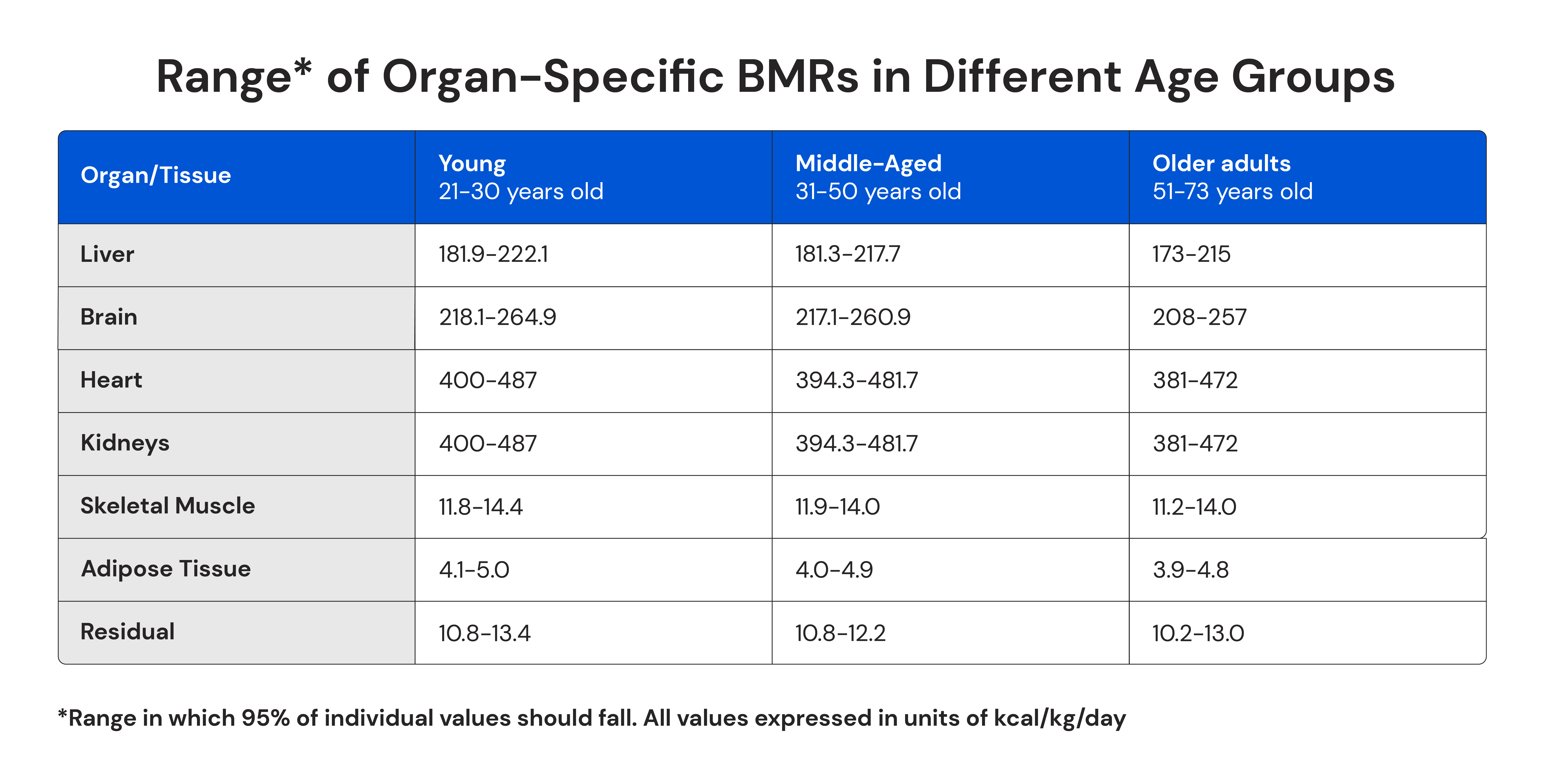
So, variability in organ-specific BMRs has a smaller impact on the overall variability of whole-body BMRs than variability in relative organ mass, but the impact is still notable. Here’s some very rough back-of-the-napkin math, and the assumptions underpinning it:

1. If you know the mass of each organ, and the organ-specific BMR of each organ, you should be able to estimate BMR more-or-less perfectly (with allowances for measurement error).
2. The limits of agreement for good BMR equations span a range of ~700-850 calories, give or take.
3. When accounting for variability in organ mass, Wang and colleagues were able to estimate BMR with limits of agreement spanning a range of just ~300 calories.
4. There’s always going to be some prediction error, simply due to measurement error. Let’s just assume that basic measurement error would account for limits of agreement spanning a ~100-calorie range.

Given those assumptions, about 100 calories of variability is accounted for by measurement error, meaning about 200 calories of variability is attributable to variability in organ-specific BMRs (thus accounting for limits of agreement spanning a ~300-calorie range in the study by Wang and colleagues). That would mean variability in relative organ masses would account for the remaining variability: ~400-550 calories.

Just to briefly recap this section:

1. When we estimate BMRs based on easily observable demographic and anthropometric characteristics, we’re tacitly assuming that organ mass scales more-or-less perfectly with body size, and that organ-specific BMRs don’t vary between individuals.
2. Errors in BMR predictions are primarily attributable to the extent to which those two tacit assumptions are incorrect.
3. Those two tacit assumptions are often quite incorrect – depending on the organ, organ masses are only moderately associated with body size, or almost completely unassociated with body size. Furthermore, an individual’s organ-specific BMRs might be up to 10% higher or lower than average.
4. Therefore, we should expect BMRs to vary considerably between individuals, even after accounting for relevant demographic and anthropometric variables.

Measurement error, regression toward the mean, and energy balance

Depending on your perspective, the figures in this article may either accurately reflect the inter-individual range of BMR values, or slightly overestimate the degree of variability.

For starters, there’s always some degree of measurement or estimation error when collecting data. Ideally, those errors will be evenly distributed (a similar amount of over- and underestimates, with over- and underestimates differing from true values to a similar extent). However, even when those errors balance out overall, the highest values are more likely to be overestimates than underestimates, and the lowest values are more likely to be underestimates than overestimates: that’s the basic idea behind the concept of regression toward the mean. In other words, if measurement and estimation error didn’t exist, you’d generally wind up with a bit less variability in your data set.

However, the degree to which variability is overstated depends on a) the reliability of the measurement, and b) the degree of intra-individual variability in the variable being assessed.

In other words, if you use a measurement tool or estimation process with poor reliability, you’re more likely to overestimate the extent of variability within the resulting dataset – since there can be large measurement errors, it becomes more likely that low values are the result of large underestimates, and high values are the result of large overestimates. Furthermore, if you’re assessing an outcome that varies considerably day-to-day, it becomes more likely that high values are the result of large upward fluctuations in the variable being assessed, and low values are the result of large downward fluctuations in the variable being assessed.

In the case of BMRs, we don’t need to worry too much about measurement error. Indirect calorimetry is excellent at accurately and reliably assessing basal metabolic rate (assuming a trained technician is taking the measurement, and subjects comply reasonably well with pre-assessment guidelines – those shouldn’t be significant concerns when a study is conducted by competent scientists). Measurement error is typically less than 1%, and repeated measures are also typically within 1% of each other.

As for the degree of intra-individual variability of BMR values…it depends on your perspective.

Over short timescales, there’s very little intra-individual variability in BMR. If you measure an individual’s BMR twice within the span of a few days, those measurements will generally only differ by about 2-4%.

However, over longer time scales, and following significant dietary changes, individual BMRs can change considerably. For instance, independent of changes in body composition, starting an exercise habit might increase your BMR by up to 5-10%, whereas adopting a more sedentary lifestyle might decrease your BMR by up to 5-10%.

Similarly, being in an energy surplus can increase your BMR, and being in an energy deficit can decrease your BMR. The classic Minnesota semi-starvation experiment illustrates this point well. Being in a large energy deficit decreased subjects’ BMRs (adjusted for changes in body composition) by about 10% after a couple weeks, and by around 25% after six months. Conversely, significant overfeeding increased subjects’ adjusted BMRs by around 10-15% compared to baseline.

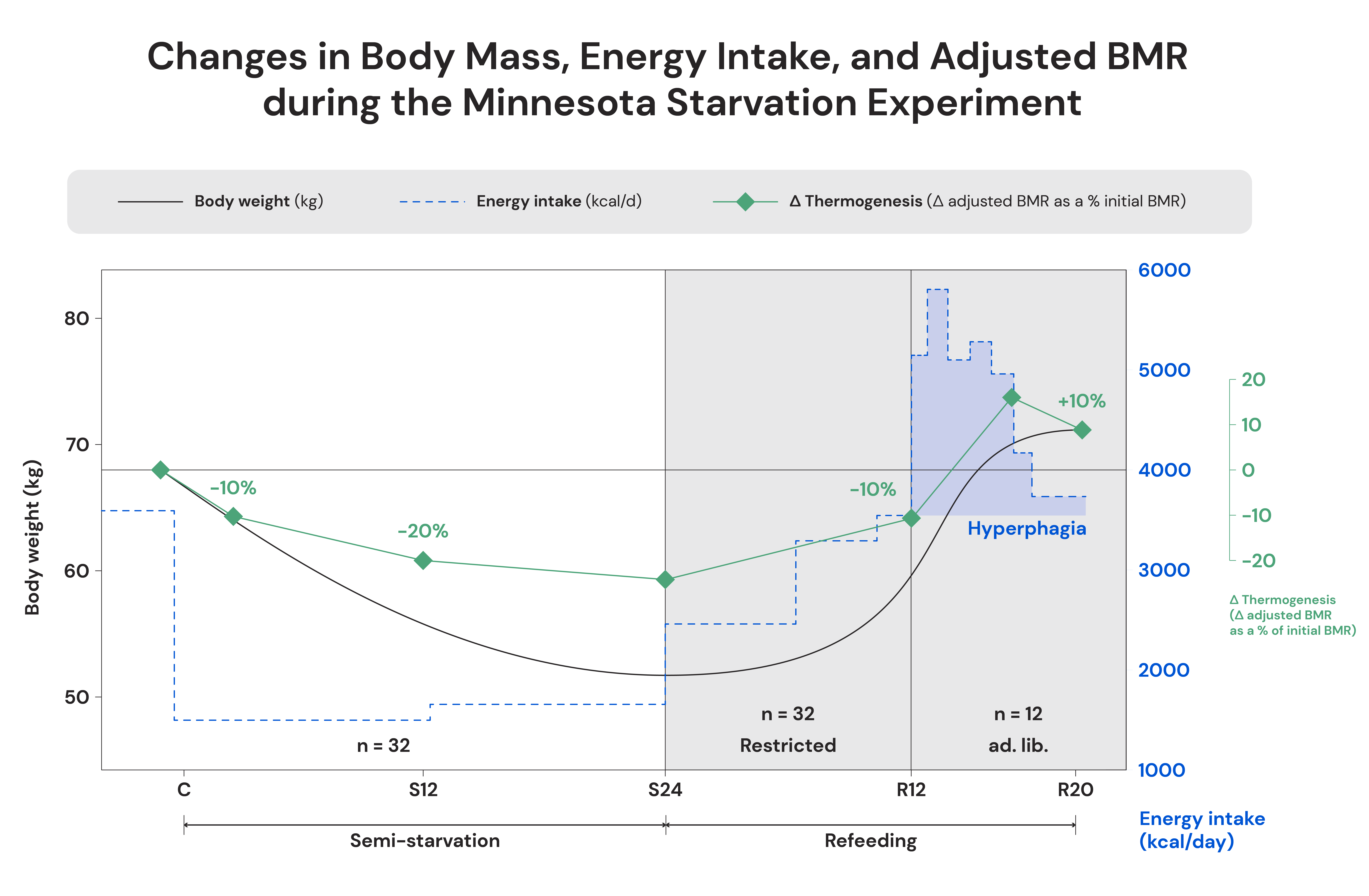
So, you could credibly argue that research on variance in BMRs and the accuracy of BMR equations might overstate the extent to which BMRs vary between individuals. If a study doesn’t ensure that all of the subjects are in neutral energy balance and exercising (or not exercising) roughly the same amount, some of the observed variability will be due to differences in exercise habits and acute energy balance, rather than “true” differences between individuals.

However, I actually don’t think that’s too much of a concern.

For starters, there’s a question of practicality. More often than not, people are interested in estimating their BMR to generate some sort of actionable insight: They want to estimate their maintenance energy needs, or generate calorie targets for the purpose of gaining or losing weight. So, they’re effectively asking “What is my BMR right now?” not “What would my BMR theoretically be if I was in perfectly neutral energy balance and exercising some standard amount?” At the time of estimating their BMR, they might be in positive, negative, or neutral energy balance, and they might be exercising a lot, or not at all. In other words, exercise and energy balance are effectively uncontrolled variables when an individual wants to estimate their BMR in the “real world,” so controlling those variables when estimating BMR variability would make the research less generalizable to “real world” situations.

Second, there is research that looks at BMR variability in more tightly controlled situations, and that research reports levels of BMR variability that comport well with the other research discussed in this article. For example, a 2017 study by Rosenbaum and Leibel aimed to examine the effects of weight loss on energy expenditure. The researchers could tightly control energy intake, because the subjects were in-patients at a clinical research center for the duration of the study. In each phase of the study, the researchers carefully adjusted the subjects’ energy intake while monitoring their weight to ensure that they were at neutral energy balance before assessing energy expenditure. So, this study fully controlled for the potential impact of acute energy balance on BMR.

At baseline, the subjects’ BMRs were reported to be 30.5 ± 3.7kcal per kilogram of fat-free mass per day. So, 95% of values should fall within 1.96 standard deviations of the mean: 23.25-37.75kcal per kilogram of fat-free mass per day. That’s a degree of variability that’s pretty similar to the variability we saw in the studies on the relative precision of BMR formulas.

Just to illustrate, you’d be predicted to have a BMR of 1500 calories per day if you had about 49.2kg of fat-free mass, given an average BMR of 30.5 kcal per kilogram of fat-free mass. However, given the reported variability (±3.7 kcal/kg), there would be a 95% chance that your BMR would fall between 1143 calories per day and 1857 calories per day. In other words, the implied limits of agreement would span a range of 714 calories for individuals with a pretty normal level of fat-free mass. That’s a slightly tighter range than we typically see in studies that don’t control for acute energy balance, but it’s in the same ballpark.

I think there’s a pretty straightforward explanation for this: If a study reporting BMR variability included a large number of subjects in extremely positive or extremely negative acute energy balance, or a large number of elite athletes and a large number of subjects on bed rest, those subjects could lead to significantly inflated estimates of BMR variability. However, most studies reporting BMR variability just recruit more-or-less normal folks, and most normal folks spend most of their time in a state roughly approximating neutral energy balance. There might be a small handful of people who are currently crash-dieting, or are in an enormous energy surplus, or are doing some other thing that leads to large acute elevations or depressions in their BMRs…but not enough to lead to significantly inflated estimates of variability.

Basically, the studies I discussed earlier might slightly overestimate BMR variability, if you’re specifically interested in knowing how much variability exists when everyone is in perfectly neutral energy balance. However, controlling for things that acutely affect BMR (like exercise and acute energy balance) would only lead to small reductions in estimated variability. Furthermore, as mentioned previously, all of those factors won’t be controlled on an individual level in the real world, so I’m not sure there’s much utility in attempting to control for them when estimating BMR variability.

What can we do about it?

After acknowledging that metabolic rates can actually differ dramatically between individuals, the next question is, “What can/should we do about it?”

I’ll start with what we shouldn’t do: We shouldn’t automatically assume that your metabolic rate dramatically impacts your ability to achieve the body composition outcomes you care about. That may seem counterintuitive, but the data bear it out. An in-depth discussion on this topic is outside the scope of this article, but you may enjoy the section of this article under the heading, “Do low metabolic rates play a major role in preventing weight loss or promoting weight regain?”

Instead, you simply need to be able to:

1. Identify whether you expend more or less energy than would be expected based on your general anthropometric, demographic, and lifestyle characteristics.
2. Quantify the extent to which your energy needs differ from the norm.
3. Adapt your diet in a manner that accounts for your unique metabolism.

That may sound complicated, but implementation is pretty straightforward. Use any standard TDEE calculator or equation to generate a reasonable initial estimate of energy needs for your goal. Then, just monitor your weight and energy intake.

Is your weight changing at the rate you want it to? If so, you nailed it! Also, that means your energy expenditure is approximately average, given your general anthropometric, demographic, and lifestyle characteristics.

Are you gaining weight slower, or losing weight faster than you want to? If so, you just need to progressively increase energy intake until your actual rate of weight change matches your desired rate of weight change. If this happens, that means your energy expenditure is higher than would be expected, given your general anthropometric, demographic, and lifestyle characteristics. Furthermore, the degree to which you needed to increase your energy intake is the approximate degree to which your energy expenditure differs from the norm. So, if you needed to increase your energy intake by 400 calories per day to gain or lose weight at your desired rate, that means you burn about 400 more calories per day than “average” for people with your general characteristics.

Are you gaining weight faster, or losing weight slower than you want to? If so, you just need to progressively decrease energy intake until your actual rate of weight change matches your desired rate of weight change. If this happens, that means your energy expenditure is lower than would be expected, given your general anthropometric, demographic, and lifestyle characteristics. Furthermore, the degree to which you needed to decrease your energy intake is the approximate degree to which your energy expenditure differs from the norm. So, if you needed to decrease your energy intake by 400 calories per day to gain or lose weight at your desired rate, that means you burn about 400 fewer calories per day than “average” for people with your general characteristics.

From there, you just need to keep monitoring and adjusting. As you gain weight or increase activity levels, your energy needs are likely to increase. As you lose weight or decrease activity levels, your energy needs are likely to decrease. As your energy expenditure changes, those changes will be reflected on the scale – you’ll start gaining weight slower or losing weight faster if your energy expenditure increases, or start losing weight slower and gaining weight faster if your energy expenditure decreases. Through this process of continually monitoring and adjusting, you can ensure that your nutrition targets are always appropriate for your weight-related or body composition-related goals.

That’s a simple enough process on its own, and MacroFactor makes it even simpler. MacroFactor effectively automates the process discussed above. It helps you a) quantify your energy expenditure, b) generate appropriate nutrition targets for your weight gain, weight loss, or weight maintenance goals, and c) adjust those targets as necessary to keep you on track as your energy expenditure changes over time.

Other methods of generating nutrition targets simply aren’t up to the task. If you just use a standard TDEE calculator, there’s not any direct mechanism to adjust your nutrition targets if the calculator’s initial recommendations are considerably too high or too low. Similarly, wearable devices that estimate energy expenditure do adjust for changes in activity levels (though they’re not particularly good at it), but don’t have any way to adjust for incorrect assumptions about your resting energy expenditure.

Ultimately, that’s why we created MacroFactor in the first place. Monitoring your weight and energy intake is still the best method for estimating your energy expenditure, adapting your diet to your unique lifestyle and metabolism, and making adjustments as things change. Anyone can do that on their own, but it can be a fairly laborious and time-consuming process. MacroFactor makes the process quick and easy.

Wrapping it up

Even after controlling for factors that influence BMR (like body composition, weight, height, age, and sex), and even without considering outliers, or people with metabolic disorders that considerably increase or decrease BMR, human BMRs cover a pretty wide range.

When you use an equation to estimate your BMR, you can use this handy heuristic: There’s a 68% chance that your actual BMR is within 200 calories of the estimate provided, and a 95% chance that your actual BMR is within 400 calories of the estimate provided. So, if a BMR equation predicts that you have a BMR of 1500 calories per day, there’s a 68% chance that your actual BMR is between 1300 and 1700 calories per day, and a 95% chance that it’s between 1100 and 1900 calories per day.

More concretely, this variability means that two people of the same height, weight, age, sex, body composition, and lifestyle could have energy needs that differ by at least 800 calories per day.

Finally, it’s time to retire the idea that BMRs don’t actually vary much between individuals when controlling for factors like height, weight, age, sex, and body composition. In a very real sense, some people do actually have “fast metabolisms” or “slow metabolisms,” independent of their general demographic and anthropometric characteristics. It might be rhetorically expedient to pretend like those differences don’t exist, but the research demonstrates otherwise.

Credit: Graphics in this article designed by infowithart.com